[HOME]   [WEB ALBUMS]   [PROJECTS]   [ARCHIVE]   [DOWNLOADS]   [LINKS]  



PROJECTS



Masers; calculation of the phase lag and period of OH masers OH127 and OH83

Several OH/IR sources were captured as described in previous projects. However these are one time measurements.

If the sources are measured on later dates, then you wil see that the amplitudes of the two peaks is varying. The reason for this is that the radiation of central star is varying. You will however notice that the amplitudes of the peaks are not varying in synchronism. The high frequency peak is leading over the low frequency peak. The reason for that can be shown in fig 1.

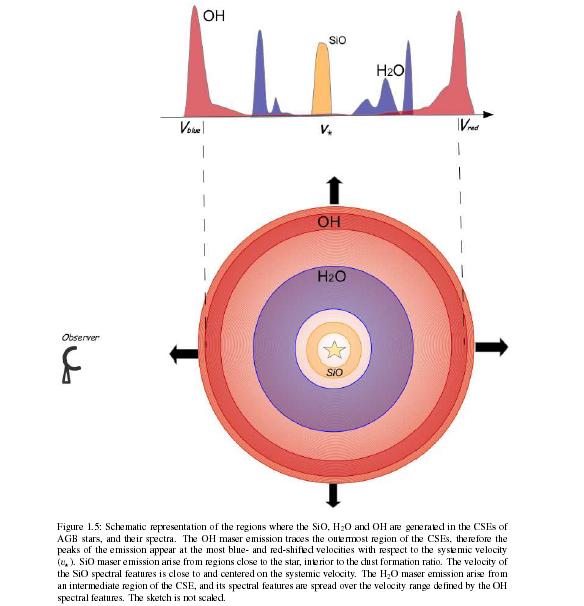
Fig.1 - OH/IR star maser emission principle. from ref1

The dying star is pulsating; expelling matter and radiating at cycling temeperatures; see the dust rings around the IR star fig1.5.

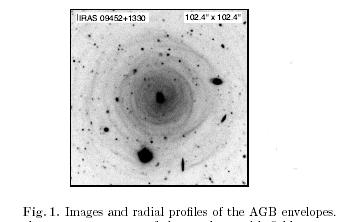
Fig.1.5 - Dust shells around old stars. from ref2

The OH shell at a far distance around the star is masing in the same ritm. However in our line of sight, the front of the shell towards us is closer to us than the shell on the other side of the star. The maser fotons have to travel in our line of sight, all the way over the extra diameter distance of the shell, before they can go on their journey to us. That takes extra time, even taking into account, that the velocity is lightspeed.

So, by measuring the phase lag between the two peaks we can calculate the diameter of masing shell of the star. Because we do not have several measurements yet, we use known graphs from puplications.

First the graph has to analysed and a table generated. The graph of OH127 and OH83 was print screen copied from ref3, ref4 and then saved as a .png.

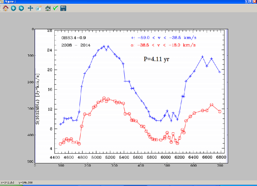
Fig.2 - Python plot of print screen dump OH83 from ref3

Next it was read into a python script here and displayed. Now when you move your mouse over plot, you get the x and y pixel coordinates. These coordinates are written in a table and read into an excel sheet.

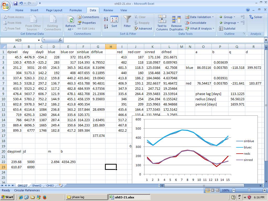
Fig.3 - Sheet OH127

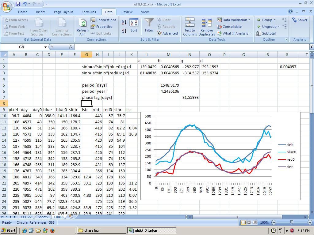
Fig.3 - Sheet OH83

You can insert a graph from the values, to check the input entered. Next you want to normalize the values because the graph is upside down. Now you want to add a table to represent the julian day instead of pixel value of the horizontal axis. Go to your orginal python graph and note the pixel value on the horizontal axis, the marker for julian day 5000. Do thesame for the pixel value of the marker for the 6000 julian day. With some algebra you can calculate m=(y2-y1)/(x1-x2), and n=y1-m*x1. With y=m*x+n you can fill the table to give the julian day value next to the amplitude. Next you would want to normalize that table too, to start it from day 0.

Now for the real job; our reasoning is that the pulsation is cyclic, so the first approximation is a sine.
The formula for the sine is y=a*sin(b*(x+q)+d.

We are going to calculate a sinewave and compare it to the real measured value. for each day cell we take the difference of the real and calculated value and write that into the next table; the least square table; (real value- cal value)^2. Next we add all the error values together. Of course, to get the best possible fit, this sum of errors values must be as small as possible. To help in the process, it is wise to show the approximation line and the real line together in a graph. When at first you estimate the variables a, b, q, and d to be 1, then the graph display is way out of line. But with reasoning the results improve.

Next, look at the least square error table; you will see that some values are very high; indicating a large difference between real and estimated value. Delete the values above 1000 from that list. Now to improve the matching further we can use the "solver" incorporated in excel. You can activate that by clicking; home, excel options, add-ins, manage add-ins go, select solver add-in ok, install. In the "data" tab, in the rihgt upper corner you will find the solver. To use it, click on "solver", next set target cell to the sum of all the least squared differences (LSD). Next select "By changing cells", and then your estimated values for a, b, q, and d, separated by a comma. Press solve, and when you are happy with the result you can keep it, or restore original values. Repeat the procedure with deleting the highest LSD and solving. Instead of varying all params, you can vary just one at a time and examen the result. Also you can alter in the solver options tab the accuracy, the iterations. etc.

Do thesame for the second table (RED). Display those lines also in thesame graph.

In the end result you will see, that a-blue and a-red representing the amplitude, are different. Also the offset d-red and d-blue are different. However, omega; b-red and b-blue must be about thesame. If not quite thesame, than calculate the mean value of these two, and fill in in both parameter cells. Recalculate with the solver the other parameters without altering the "b" value.

The total period is now; 2*pi()/b [days]; for OH83 this means a period of 4.2 year.

The phase lag is the difference between q(blue)-q(red). For OH83 this is a phase lag of 31.6 light days; that is about 22 times the diameter of our solar system.



Eventually the interstellar x-rays will break up the molecule into H and O, and that is where our oxygen is coming from.

More molecules like silicon (sand), aluminum, upto iron are fabricated and expelled by the dying star, but that is another story.



Michiel Klaassen januari 2016

ref1
ref2
ref3
ref4
ref5
python plot script