PARAC info

dish

[HOME] [WEB ALBUMS] [PROJECTS] [ARCHIVE] [DOWNLOADS] [LINKS]

project MK6 Adding more Python functions to Cfrad post processing

Introduction.
The extra functions are often just a few script lines, so it is not usefull to publish a new version of a plot script with every new line. We just take the standard plot script here.

http://parac.eu/cfrad-plot-eng.zip

and indicate where to insert the new fuction. You have to find the equivalent location in your own script.

1. Average multiple spectra lines.
If you have a stable measurement, you could wish to integrate the signal of the source longer than 5 minutes.
Average of a number of 5 minute spectra and save sum file to disk for later use.
Insert after original line 189
#---------------------------------
sumsets=np.zeros((2048)) ;
sumf=3#sum spectrum number from
sumt=23#sum spectrum number to
for sets in range (sumf,sumt):
sumsets=sumsets+outsets[sets]
sumsets=sumsets/(sumt+1-sumf)
np.savetxt(filename+"sum"+str(sumf)+"-"+str(sumt)+".txt",sumsets)# save sum file
#---------------------------------

You can add the average spectrum sum at the bottom of the overview graph.
Insert after original line 192
#---------------------------------
ax.plot(f-Sf,sumsets,linewidth=1)#
#---------------------------------

all lines shift correction

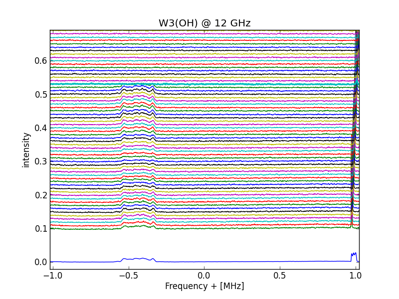
Adding multiple 5 minute spectra and plot result

2.Prepare for contour plotting or fits file generation.
To show a contour graph, all the nrad files have to be corrected for the bandpass curve.
Also the spectra base lines have to be normalized; that is; the baseline drift has to be compensated.
If not, you get jumps in the contour lines. See project MK5 to post process the contour graph.
Insert after original line 187
#-------------------------------
   offsetcor=1-((data[50]+data[60]+data[1990]+data[2000])/4)#line space normalizing
   data=data+offsetcor
   np.savetxt(filename+str(sets)+".tct",data)#csv preparation. to disable; place # at start of line
#------------------------------

normalization no

No Normalization

normalization yes

With normalization

3. Compensate slanting of the baselines.
Because of temperature drift or meteo differences over a long time, the baselines can start slanting.
This can be compensated . Note that the absolute baseline value is changed by this action, however for frequency comparations this has no effect.
Insert after original line 184
#-------------------------------------
   beg=np.mean(data[180:220]#or choose another start value
   eind=np.mean(data[1828:1868]#or choose another endvalue
   for i in range (0,2048):
       data[i]=data[i]+i*(beg-eind)/1648#correct z axis slanting
#-------------------------------------

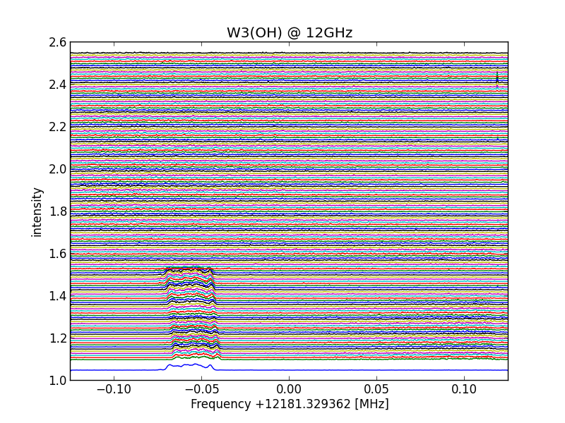
slanted-corrected

W3(OH-12GHz-slanted and corrected

4. Plot all spectra with 2048 BINS as x-axis.
This can be usefull when you want to know in which bin an amplitude effect took place.
Insert after original line 207
#------------------------------------------
fig=mpl.figure(2)
ax = fig.add_subplot(111)
#ax.plot(sumsets,linewidth=1) #average
for i in range (vans,ms+1):
ax.plot((outsets[i]+offsets[i]))
ax.set_title('signal')
ax.set_xlabel('BIN')
ax.set_ylabel('Intensity')
mpl.show()
#------------------------------------------

5. Compensate frequency drift; because of xtal drift.
Use option nr 4 to plot the spectra.
Point with your mouse at a distinct feature of the source curve (first line) and note the bin number=x
Next select the latest line of the source curve for which you want to compensate.
Point again to thesame feature on that last line and note the bin number=y
Count the number of lines between the two selected lines=z.
a=abs(x-y)/z
Remove one of the '#' to select correction of the top to the left or the right.
Insert after original line 164
#------------------------------------------
   for set in range (vans,int(sets*a+0.5)) : #shift: a=abs(x-y)/z
       for q in range (1,2047):
#           data[q]=dat[q+1] #shift top to left
#           data[2048-q]=data[2048-q-1]#shift top to right
#------------------------------------------

all lines w3-av

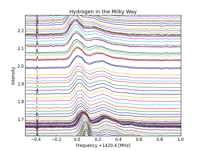
temperature frequency drifted lines

all lines shift correction

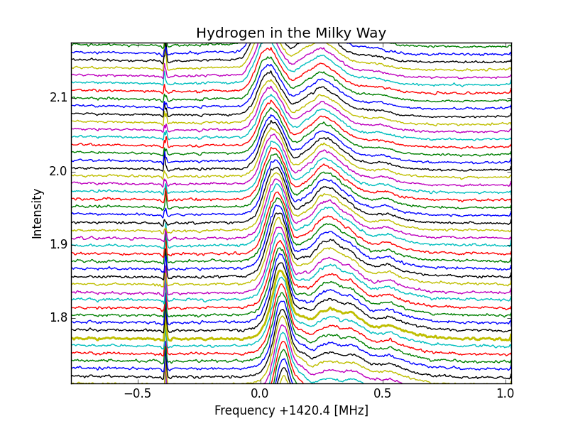
All lines shift corrected

6. Reverse spectrum.
There are several ways to do that, but I choose on obvious one.
Replace line 202 with
#------------------------------------------
ax.set_xlim( Sf, -Sf)
#------------------------------------------

Reverse X scale

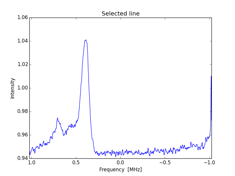
X scale corrected curve

7. Adding a second scale; for instance; VLSR.
For neutral hydrogen;
frVLSR=(3e8*(1-(obsfreq-bw/2)/restfreq)/1000-LSR
toVLSR=(3e8*(1-(obsfreq+bw/2)/restfreq)/1000-LSR
restfreq=1420 405 752 Hz
observation frequency =1420 000 000 Hz
bandwidth=2048000 Hz
LSR=Velocity of the Local Standard of Rest of the earth; this includes rearth own rotation and rotation around the sun.
This value can be calculated from;
http://neutronstar.joataman.net/technical/radial_vel_calc.html
This value varies between + and - 30 km/s; As a first appoximation; LSR can be set to 0.
Insert after original line 206
#------------------------------------------
ax2 = ax.twiny()
ax2.set_xlim( frVLSR, toVLSR)
ax2.set_xlabel('VLSR [km/s]')
ax2.set_title('Milky Way - 16-6-2014', y=1.07)
#------------------------------------------

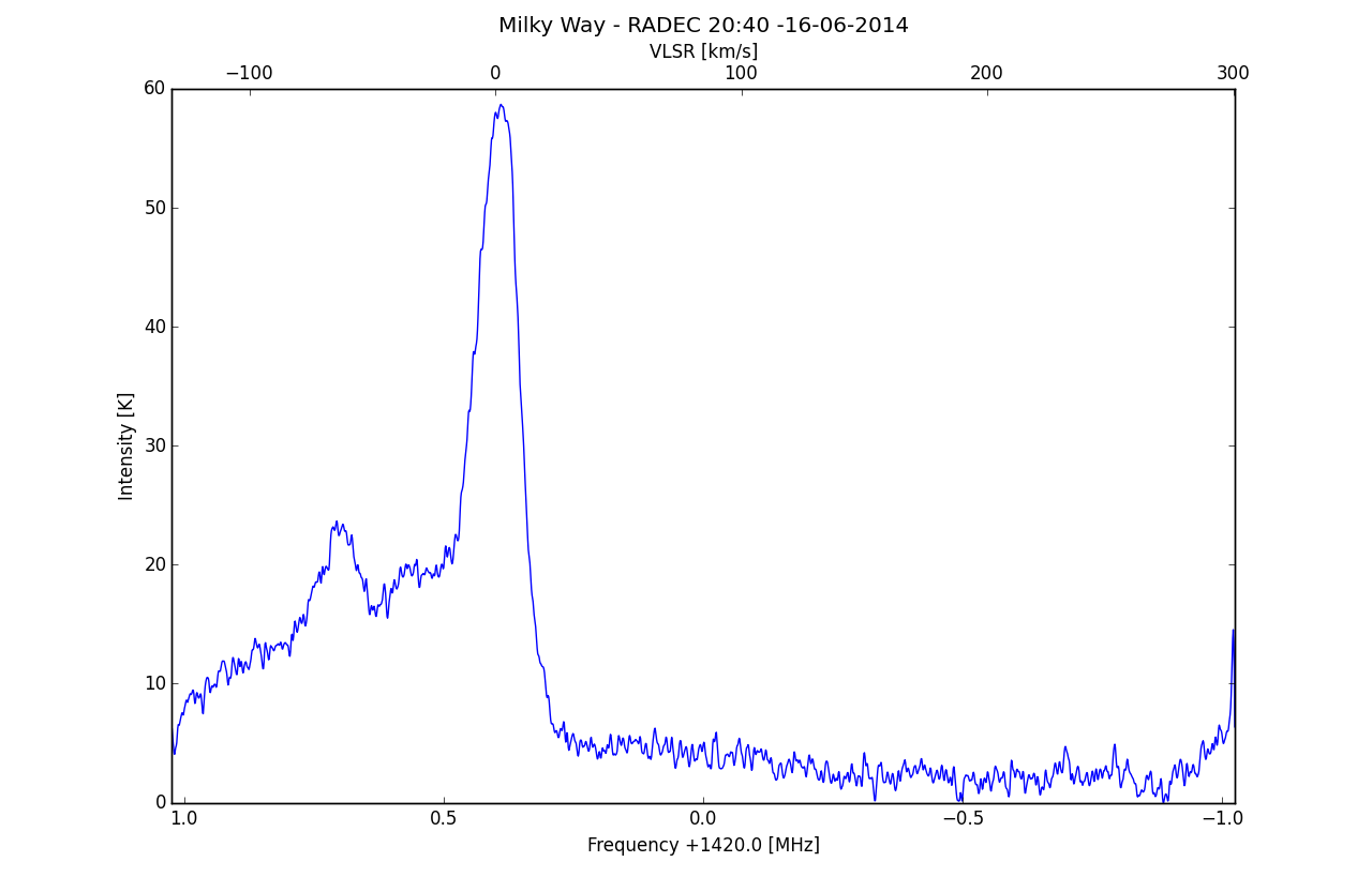
Added second X scale

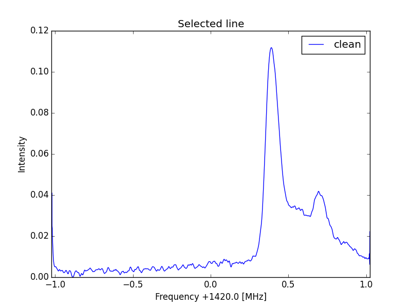
8. Change the reference level from 1 to 0.
Replace line 141 with
#------------------------------------------
ax.plot(f-Sf,(raw4)-np.min(raw4), linewidth=1,label='clean')
#------------------------------------------
Or select a 'no signal' region and calculate an average reference value to subtract
#------------------------------------------
ax.plot(f-Sf,(raw4)-np.mean(raw4[300:400]), linewidth=1,label='clean')
#------------------------------------------

9. RFI suppression.
9.1 Valley finding.
In the graph, successive low points are connected, and so pieks are cutt off.
Disadvantage is ; loss of resolution.
The gap to bridge can be set from 1=no gap to 50= large gap, default=10

Insert after original line 125
#------------------------------------------
C=0
D=data[0]#scan start
for i in range (1,2047):
   if data[i] <= data[i-1] and data[i]<data[i+1] and (i-C)<10: #dan valley
       dalval=data[i] # found valley value
       for n in range (1,(i-C)):
           data[C+n]=(n*(dalval-D)/(i-C))+data[C]# linear interpolation
       D=dalval
       C=i
   elif data[i] <= data[i-1] and data[i]<data[i+1]:
       D=data[i]
       C=i
#------------------------------------------

Insert after original line 53 or 164
#------------------------------------------
   C=0
   D=data[0]#scan start
   for i in range (1,2047):
       if data[i] <= data[i-1] and data[i]<data[i+1] and (i-C)<10: #dan valley
           dalval=data[i] # found valley value
           for n in range (1,(i-C)):
               data[C+n]=(n*(dalval-D)/(i-C))+data[C]# linear interpolation
           D=dalval
           C=i
       elif data[i] <= data[i-1] and data[i]<data[i+1]:
           D=data[i]
           C=i
#------------------------------------------

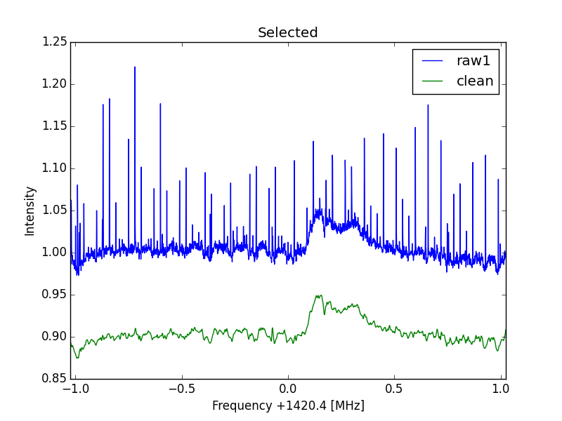
RFI suppression

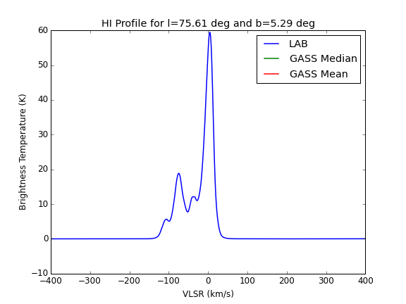
10.Vertical Scale calibration.
Point telescope to strong H1 source like direction RA 20H, DEC=40deg.
Use https://www.astro.uni-bonn.de/hisurvey/profile/ and also fill in the beam of the telescope to get the profile.
Note the peak value of the unibonn curve =UB
Note your raw peak value=RV
Gain correction: GC=UB/RV
Insert after original line 150
#------------------------------------------
fig=mpl.figure(sets)
ax = fig.add_subplot(111)
ax.plot(f-Sf,GC*(raw4-np.min(raw4)), linewidth=1)
ax.set_xlim( -Sf, Sf)
ax.set_title('Selected line')
ax.set_xlabel('Frequency +1420.4 [MHz]') #
ax.set_ylabel('Brightness Temperature [K]')
mpl.show()
#------------------------------------------

Standard selected line

Standard curve

Reference curve

Y-scale corrected

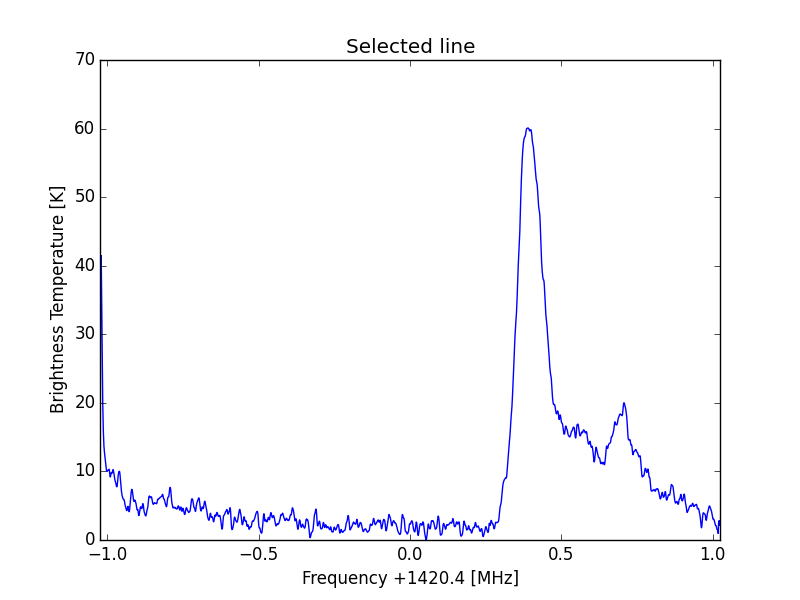
Y scale corrected curve

11. Intensity as a function of time.
The spectrum consists of 2048 bins; each bin can be selected as a time signal.
It will be more easy to choose a bin when option 4 is used.
More bins can be chosen also to form an averaging signal.
Insert after original line 207
#------------------------------------------
data=np.zeros((ms+1,2048)) ;
sign1=np.zeros((ms+1,1));#signal 1 of possible 2048 signals
reflow=np.zeros((ms+1,1));#reference
for n in range (0,ms+1):
   data[n] = np.loadtxt(filename+str(n)+".txt")
   data[n]=data[n]*bpcorr
   for k in range (1407,1408):# select bins of interest
       sign1[n]=sign1[n]+data[n,k]
   for k in range (500,510): #select quiet part of spectrum (in bins)
       reflow[n]=reflow[n]+data[n,k]
sign1=sign1/1
reflow=reflow/10
fig=mpl.figure(2)
ax = fig.add_subplot(111)
ax.plot(516*((sign1-reflow)-np.min(sign1-reflow) ) )#
ax.set_title('Milky Way drift scan')
ax.set_xlabel('*5min from start')
ax.set_ylabel('Brightness Temperature [K]')
mpl.show()
#------------------------------------------

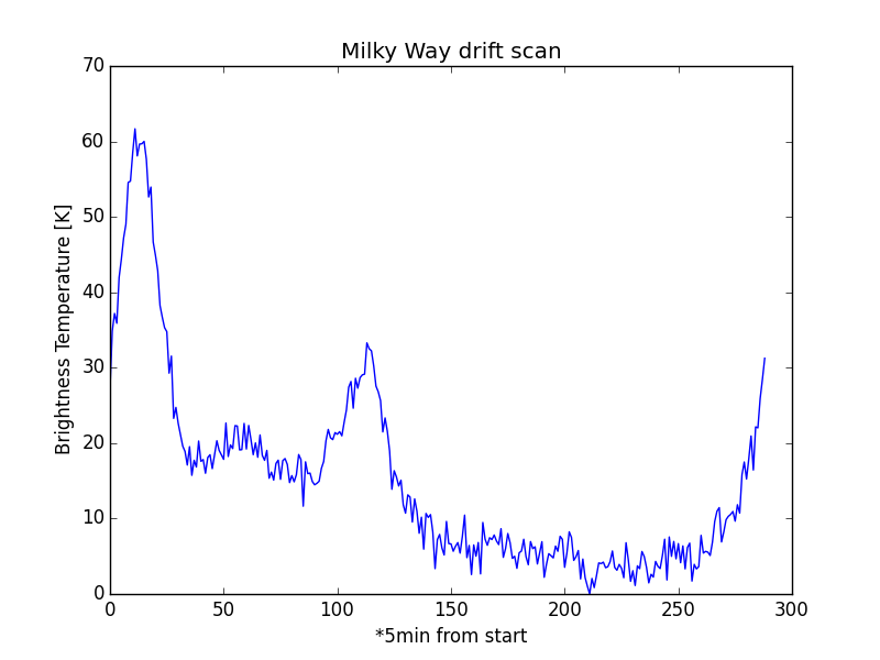
Brightness versus Time

Michiel Klaassen 03mrt2020