[HOME]   [WEB ALBUMS]   [PROJECTS]   [ARCHIVE]   [DOWNLOADS]   [LINKS]  







project MK5: Post processing radio astronomy data; plot

The data you have captured with CFRAD2.exe or other programs can be postprocessed with python or excel. First we will process it with excel to give you an idea of the procedure.

Excel post processing

In the capture example we have given 2 result files; nrad29 is was captured as the dish was pointed to the source, and nrad180 was taken 12 hours later, when not pointed to the milkey-way as a reference. Two example data files measured with an 80cm dish can be downloaded from here;

nrad-29.txt  

nrad-180.txt  

To have a look at it you can open it in an editor; we use free "editpad light". The 2048 values are the bin values of successive frequency bands. Also you see that the decimal seperator is a dot. Excel in some countries wants to see comma's, so to change that go to edit, select all, now go to search, and click prepare to search. In the left bottom corner two windows are visible; put in a dot left and a comma right. Now go in the search tab to replace all; done. The list is still highlighted, now; rightclick copy. Startup excel and click on the left most colomn and right click paste. Do the same for the second file; the reference file; nrad180.

If you insert a graph now and plot the two colomns you will get a passband curve. We can correct that by making a third colomn where we divide colomn A/B. Next, in colomn C we amplify the graph and subtract a constant value to bring it into the window. Now you can insert a graph, and it would be similar to the example.

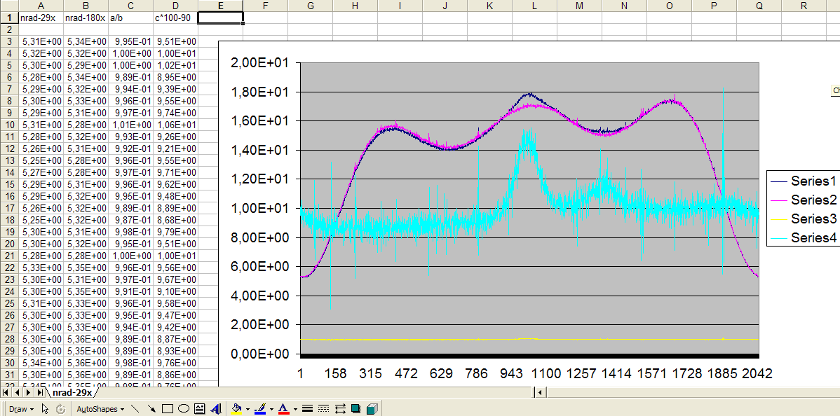
Fig.1 - Excel result.

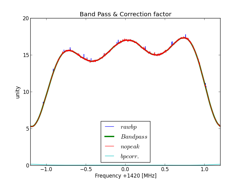
Fig.2 - Python plot2 band pass.

And some details where you can see that the anti peak function is working.

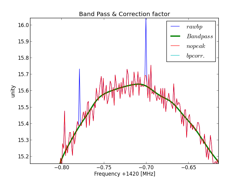
Fig.3 - Python plot2 peak removal.

This is the function we will use later to correct the received signals with.

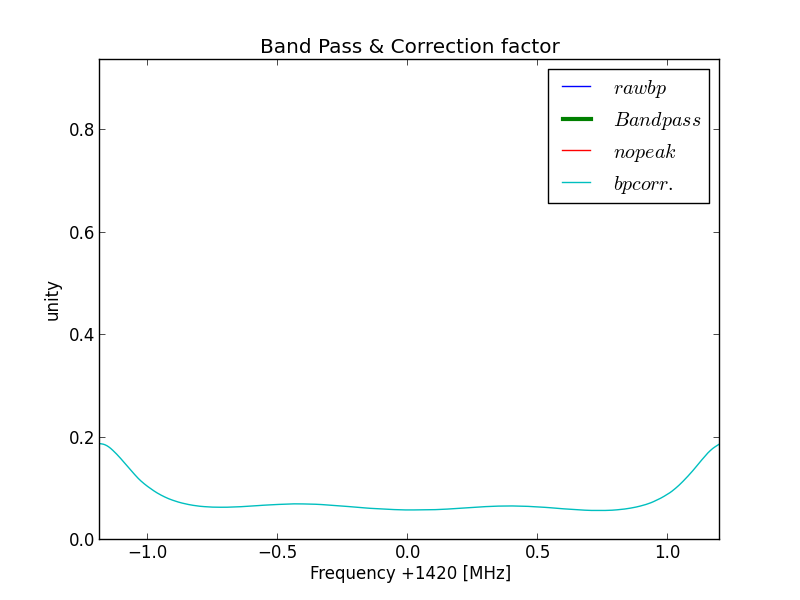
Fig.4 - Python plot2 band pass correction.

You can zoom in on any part of the graph by selecting the fifth icon from the left. When you are done, you can click the X in the right upper corner. The script continues the program and halts to display the "selected 5 minute" measurement. It gives thesame result as the A/B funtion in excel. Now we see the actual hydrogen line curve.

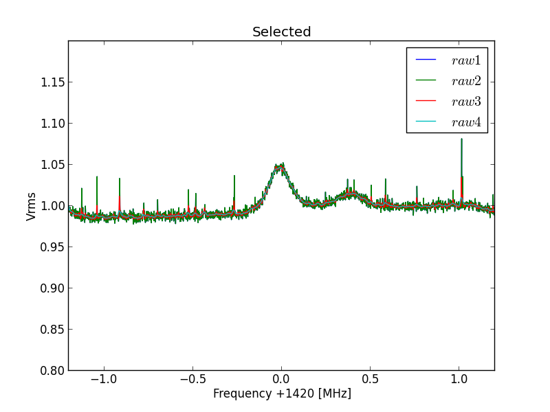
Fig.5 - Python plot2 select curve 29.

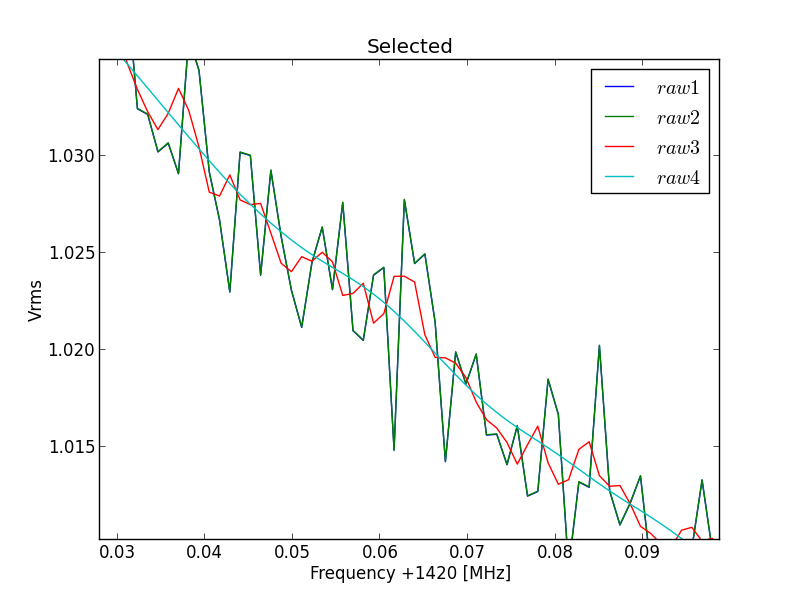
Fig.6 - Python plot2 selected curve 29 detail.

Click on X to proceed.

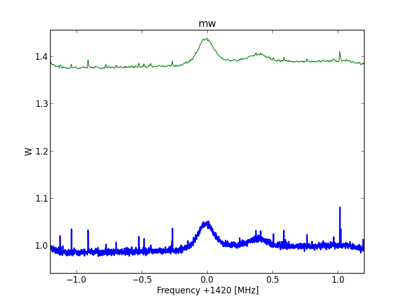
Fig.7 - Python plot2 final20b.

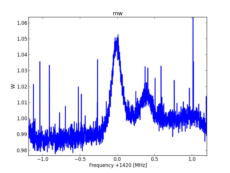
Fig.8 - Python plot2 raw detail.

Click on X to proceed.

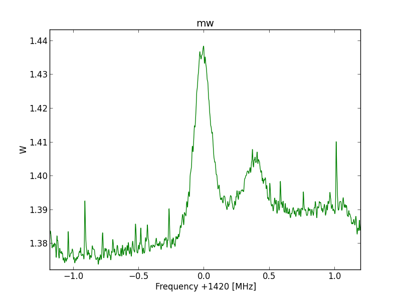
Fig.9 - Python plot2 final20 detail.

The full 24 hour session



The full 24 hour data (288 data flies) can be downloaded from here; cfrad288.zip   Also the python sript is added into the zip file. Python is a free platform used in scientic and universities. It is fast and has the feel of old "Basic". The version used by us is Python-xy and can be found here https://code.google.com/p/pythonxy/wiki/Downloads; install it. Included is the an editor called "Spider".

I the editor go to the folder with the unzipped files and , open the file cfrad288.py, and run it. The reference for this 24 hour run is taken from the quiet part of the scan, this is not what we normal do, because everywhere there are hydrogen background signals, but for the moment this is easy. So the the scans 180 to 190 are taken as "zero" reference. The mean value of these scans are taken, which gives a smooth line like;

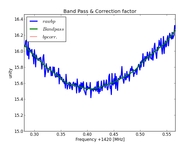
Fig.8 - 288 band pass curve detail.

In another project we can also show the use of a polynome with multi-coefficients to fit the curve. making it even more smooth.

For now we use this curve to inverse multiply the rest of the measured files with. The script continues when the top right X is pressed. Next the selected curve is shown. Here we can judge the script lines we think of and we do not have to wait for the processing of all the files.

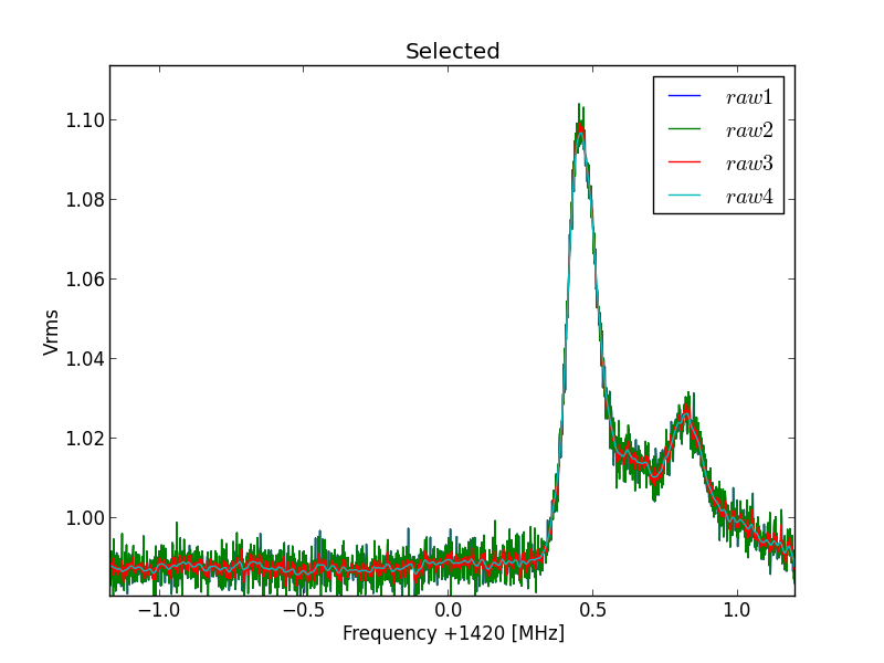
Fig.8 - 288 selected file detail 01.

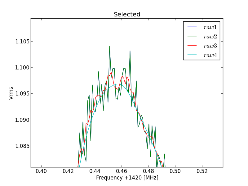
Fig.8 - 288 selected file detail 02.

If done press X again; the complete 288 files are now being processed.

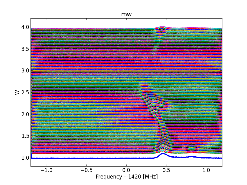
Fig.8 - 288 all scans.



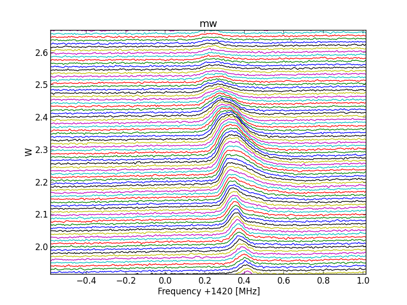
Fig.8 - 288 detail 01.



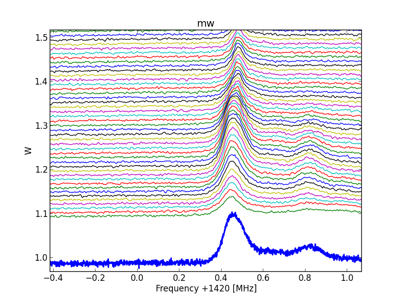
Fig.8 - 288d 02.



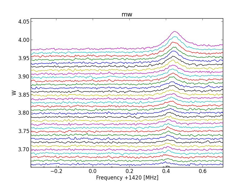
Fig.8 - 288 detail 03.

Michiel Klaassen nov-2014



CONTOUR plot of the Cfrad files

It has taken some time, but now I have found an more easy solution to generate a contour map with python. So, now I can share this method with you also.

First, the band pass corrected nrad files (the spectra), which normally are line plotted, have to be saved to disk. This can be automated when one script command line is added to the cfrad plot script like this;

np.savetxt(filename+str(sets)+".tct",data)# csv preparation

Put it at the end of the 'series' block.

Now if you run the modified plot script, all the extra .tct files will be written to disk.

Next these .tct files have to be packed into a csv file with the csv-maker.py script.

cvs-maker.py  

In this script you can alter the values for the lines to use; so instead of 0 to 288 you can choose 100 to 200. (frcycle=100 tocycle=200) Also you can alter the frequency range (in BINS) to incorporate. Normally 0 to 2048 is used. However if the beginning or the end of the range is warped you can choose to limit the frequency range to values from .. and to ...(fbin=..,tbin=..)

Let the cvs-maker script run. It will take a while; for 289 files about 9 minutes on a modest machine. You can check the produced .csv file; its about 18MB. When you open it with an editor like 'edit pad lite', you will see 3 columns; bin-nr, spectrum-nr, intensity-value.

Next you can use all kind of tools to plot this csv file, but you can also use 'plot-contour.py'. If you have altered the frequency range bins, then you must do some homework to adjust the frequency contour scale also.

plot-contour.py  

Running this script takes about 1 minute. Below are some contour examples of the nrad288.zip files from the parac.eu download page

One of the variables you can modify in the plot script is the resolution of the levels. In the graphs you see the difference between 10, 50, and 500 levels.

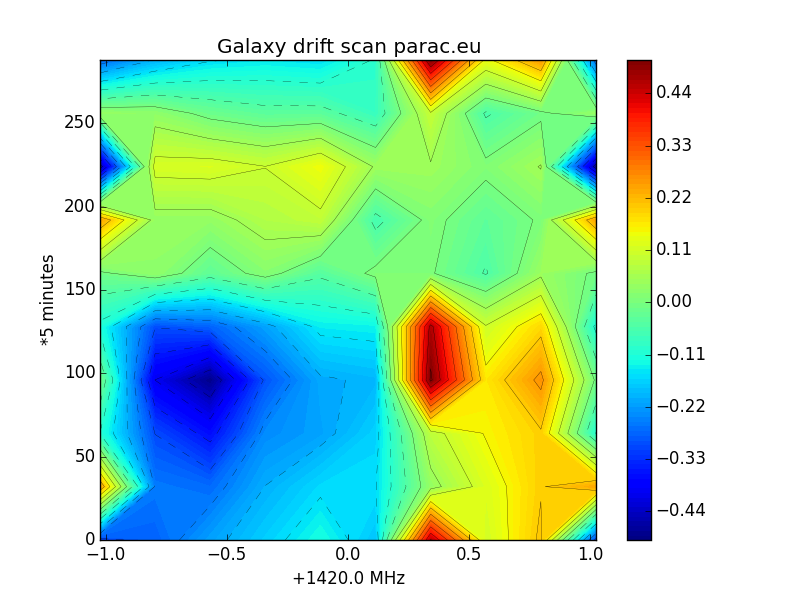
Fig.9 - galaxy scan low resolution.





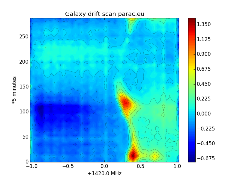
Fig.10 - galaxy scan medium resolution.





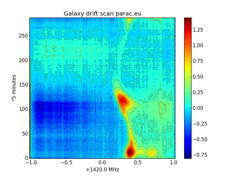
Fig.11 - galaxy scan high resolution.

Michiel Klaassen feb-2020





9. 'Flexible Image Transport System' or FITS.

It is also possible to convert the Cfrad files into a .fits file.
There are numerous packages to manipulate a fits file see:
https://fits.gsfc.nasa.gov/fits_viewer.html
I just tried one program; 'fv' or 'fits view'; a FITS file viewer and editor (supports FITS images and FITS tables)
You can plot just one spectrum or you can can plot all spectra and display it as a heatmap, contour map or perhaps more.
Also you can make a profile line anywhere in the map and display the intensity graph.

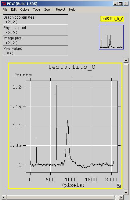
Fig.9 - 1 selected spectrum.

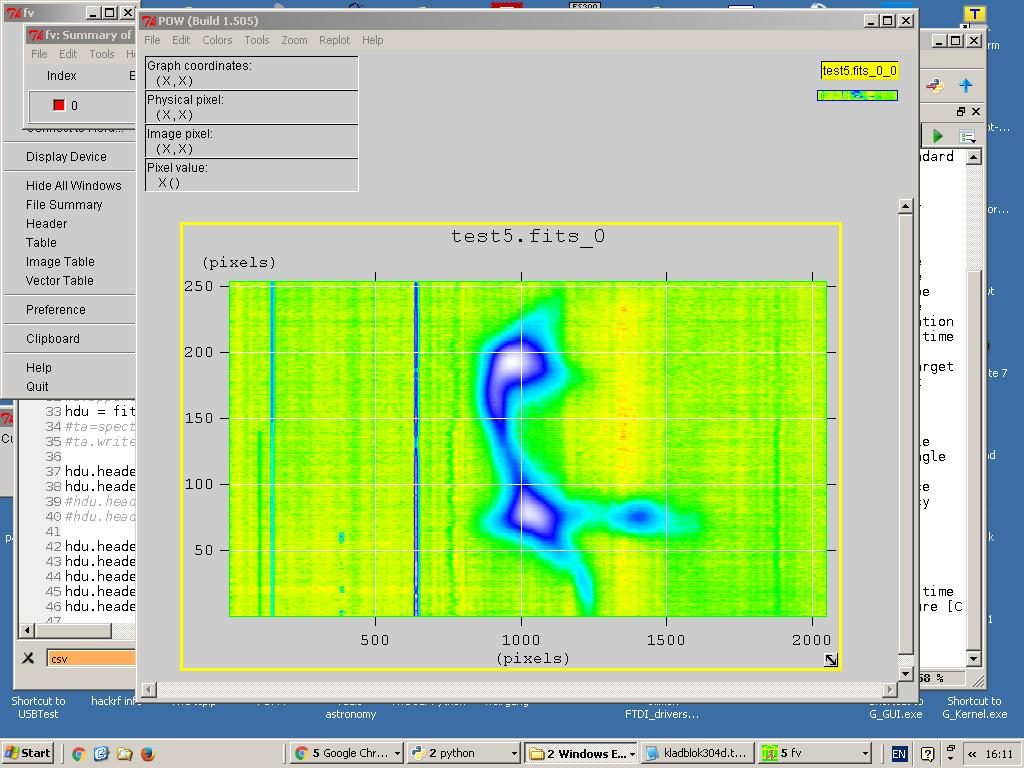
Fig.9 - Multiple spectra.

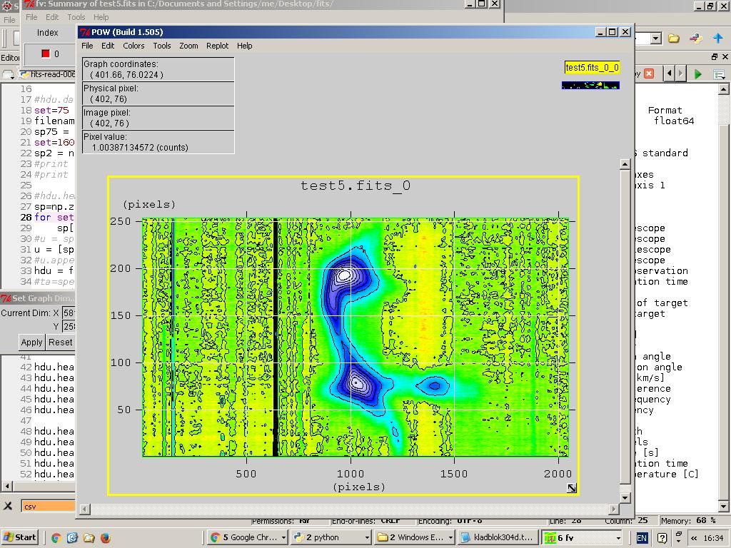
Fig.9 - Contour plot.

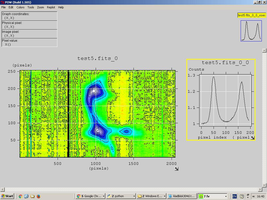
Fig. - profile selection.

As a preparation, the original nrad.txt files have to be bandpass corrected and preprocessed (rfi suppressed etc).
The intermediar results are written as .tct files. See the description on how to do that in project http://parac.eu/projectmk6.htm item nr 2.

Next, you have to install the latest astropy version, or running astropy-v103 from here.
astropy103: Astropy version 1.0.3.11-11_py27

Load the cfrad-to-fits-01.py script here into your (spyder) editor.
You can modify the hdu.header lines to your own liking or purpose.

One spectrum processing into a fits file.
In line 14 you can select 1 file to be converted into a fits frame.
To process that you have to remove the # from the beginning of line 24.
Place a # at the beginning of line 25 to disable that instruction.

Multiple spectra processing into a fits file.
In line 18 you can put the number of sequential nrad files to be processed; maximum is 288.
Next, remove the # character from the beginning of line 25.
Place a # at the beginning of line 24.


Finally, run the fits generating script in the same directory as the .tct files and the fits file will be generated.
As a comparation, here is also a test.fits file here.


reference: Astronomical Image Processing System; AIPSMEM117.pdf here
See also: http://www.aips.nrao.edu/index.shtml#FITS


Michiel Klaassen march 2020