[HOME]   [WEB ALBUMS]   [PROJECTS]   [ARCHIVE]   [DOWNLOADS]   [LINKS]  







project MK4: CFRAD2.exe; Capture and Fast Fourier Transform Radio Astronomy Data with a RTL dongle (Software)

For those amateurs who want to try to receive the hydrogen line signals with a RTL dongle on a windows machine; here is a method to do so. This program captures and calculates FFT and add them in a file; 100000 spectra are avaraged in 5 minutes Sharp# is used for the settings.

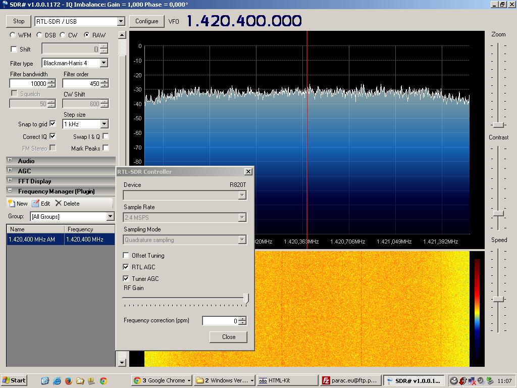
Fig.3 - Sharp# screen.

Download the zip file from here CFRAD2.zip  

1. You need to unzip the CFRAD file to a folder and copy the libusb-1.0.dll to the systems32 folder.

2. Start your Sharp# program, select your RTL usb dongle and select play.

3. You can select any sample rate, AGC settings etc for your need.

4. Bring up the task manager by pressing ctrl alt delete.

5. Go to the window "processes" tab in the task manager.

6. Right click SDRsharp.exe and click "end process", and again "end process"

7. Go to your cfrad2 folder and start cfrad2.exe

Immediately a raw file is written; you can open it with an editor and check the first two values in the file. These values are the highest and lowest value the program received from the dongle. minimum is 0 and maximum is 255. The middle value is 127. Best is, to use the whole range of the a/d converter; so a range of 5 to 250 is preferred. If way off, add more or less gain to your system.

After 5 minutes the first FFT .txt file will be written in the same folder as the cfrad application was located. There are 2048 bins. Dependend on your setting of the SDR# sw, these bins cover the selected bandwidth (quad mod). Example: If you selected 1024MS/s Quadmod, then the output range is 1.024MHz, and each bin is 1024/2048=500Hz wide. In total 288 text files will be written in 24 hours.

The output value is rms voltage.

You can stop the program any time by terminating it in the taskmanager.



Efficiency

The most important specification for FFT programs is that they produce as much spectra/s as possible. So best is to use a fast machine and not waste PC time on other tasks. This can be checked in the taskmanager; the processor core must be loaded 100%, and your fan has to ramp up after some time.

A quad core 1.8GHz, 2.5GB machine was used with W7 os.

Sample rate	number of obtained spectra	efficiency	real integration time
[MS/s]	in 5 minutes	[%]	minutes
3.2	100645	20	1
2.048	100500	34	1.7
1.048	96057	63	3.15
0.25	36620	100	5

Fig.1 - Efficiency Result Table.

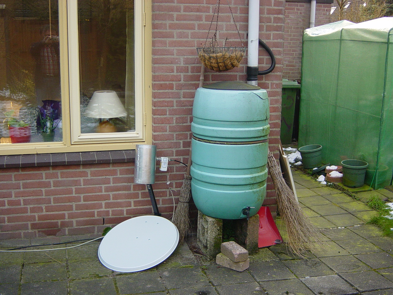
Fig.2 - Even a 55x60cm dish can be used for neutral hydrogen detection.

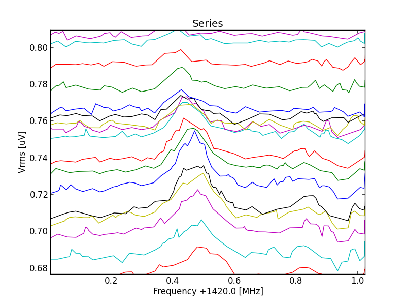
Fig.3 - Measured with a 55x60cm offset dish and python postprocessing.

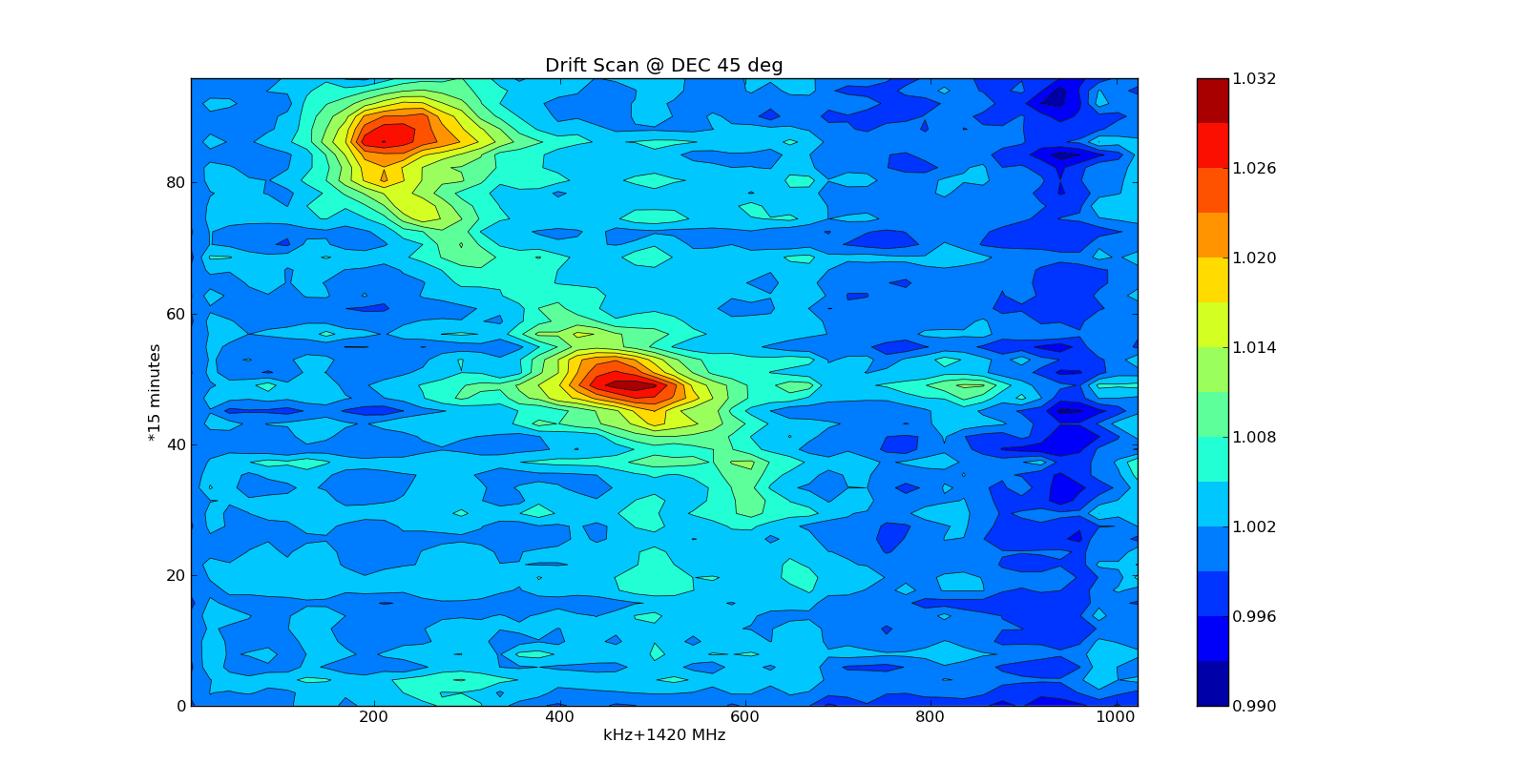
Fig.4 - 55x60cm dish contour.

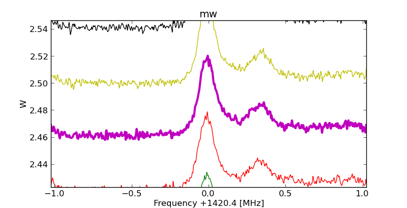
Fig.5 - Measured with an 80cm offset dish and python postprocessing.

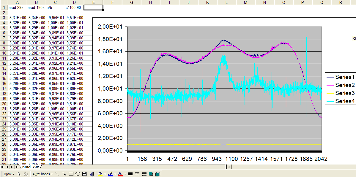
Fig.6 - Measured with an 80cm offset dish and excel postprocessing (no filtering applied yet).

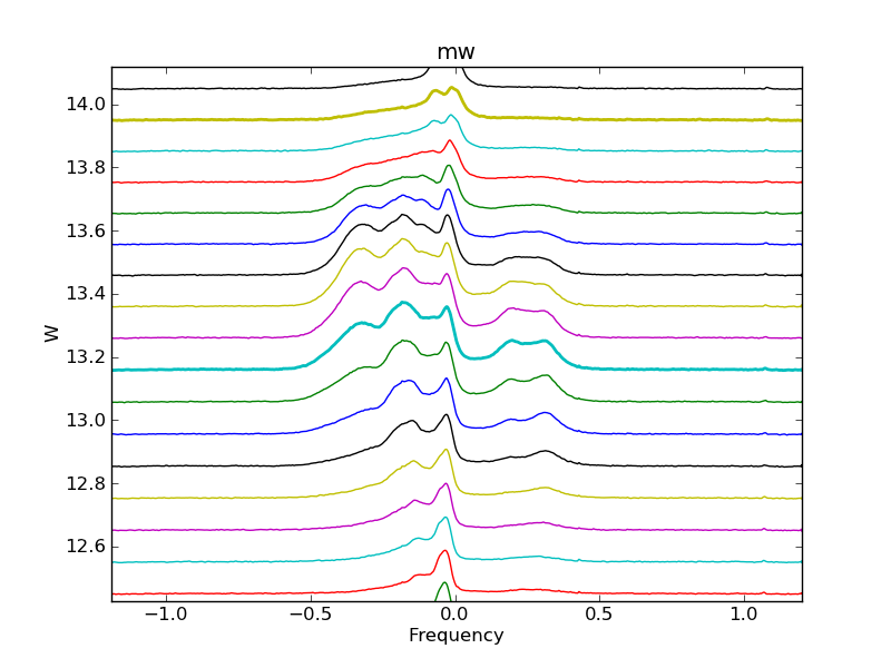
Fig.7 - measured by Hans Smit with his 3m dish .