[HOME]   [WEB ALBUMS]   [PROJECTS]   [ARCHIVE]   [DOWNLOADS]   [LINKS]  



PROJECTS



Project MK23: Complex object W3(OH) at methanol line CH3OH at 12.178 GHz

Part 1


It is known that methanol is also maser transmitting at 12.178595 GHz.

This frequency lies in the standard Astra LNB range 10.70–12.75 GHz. So, I decided to try to detect it. Some specs of the LNB are:

Voltage	Tone	pol.	Freq.input	Local.Osc	Freq.output
[V]	[kHz]	[V/H]	[GHz]	[GHz]	[MHz]
13	0	V	10.70-11.70	9.75	950-1950
18	0	H	10.70-11.70	9.75	950-1950
13	22	V	11.70-12.75	10.60	1100-2150
18	22	H	11.70-12.75	10.60	1100-2150

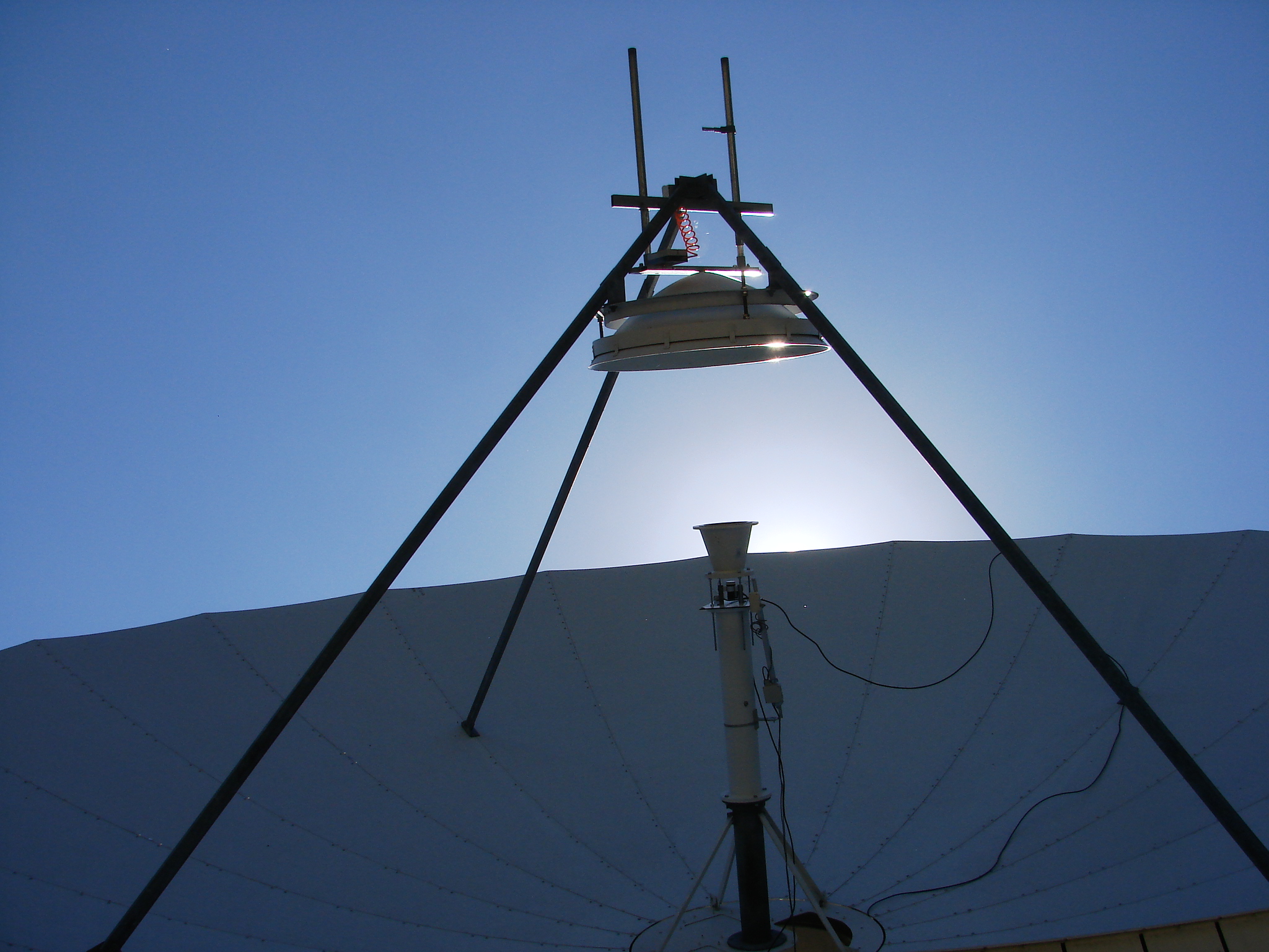
Fig.1 - Airy interface between horn and LNB

The expected output should be; 12.178595 GHz - 10.6 GHz= 1.578595 GHz, and this is in the range of the RTL sdr dongle.

Small problem is that the LO frequency is not exact or stable. Normally the TV receiver can adjust this because the signals are strong.

Another small problem is that the sky frequency is higher because W3() is approaching us.
I used my earlier W3(OH) measurement as a reference, because these OH clouds have the same velocity toward us.
I used the ratio from 1.6GHz to 12.1GHz and adjusted the dongle receiver frequency to 1.581 GHz.
So, the central frequency in the receiver is 12.181 GHz


For the software I used cfrad2.exe again; giving me every 5 minutes the average of 100000 FFT spectra.
The first two X5 minutes the dish was off target and this result is used as a reference; lines green and red.
In stead of subtracting the base line as I see some amateurs do, I divide the on target result by the off target result.
This is done in python; all the software is free and can be downloaded from parac.eu


Because the LNB LO is not stable, the output shifts in frequency over time/ambient temperature, so if you average a lot of data blocks, then the result will be smeared out and disappears.
The end result here is averaged over 16X5 minutes.

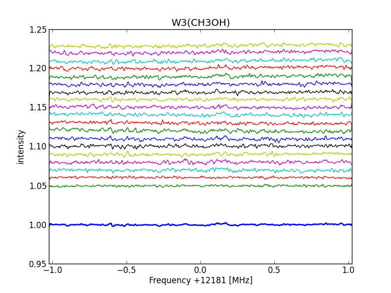
Fig.2 - Overview W3(OH) @12GHz

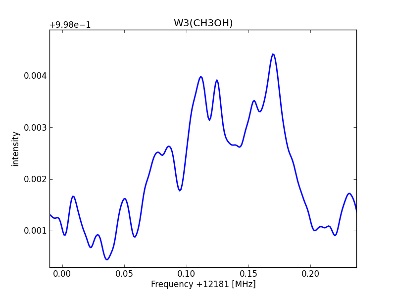
Fig.3 - Sum of 16x5minutes integration @12GHz

The literature result gives a horizontal flipped over notation

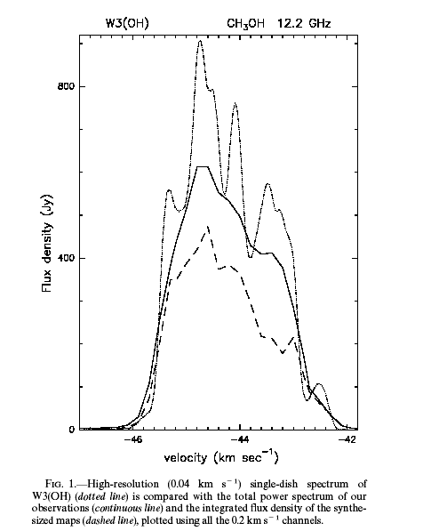
Fig.4 - W3(OH) @12GHz from literature; high frequency side is on the left

Part 2

Given the advice by Harke and Marcus I purchased an Avenger LNB with pll control.
The frequency stability of this LNB is much better, however there still is an amplitude variation somewhere.
Also I fully mounted the original horn; no airy interface anymore.

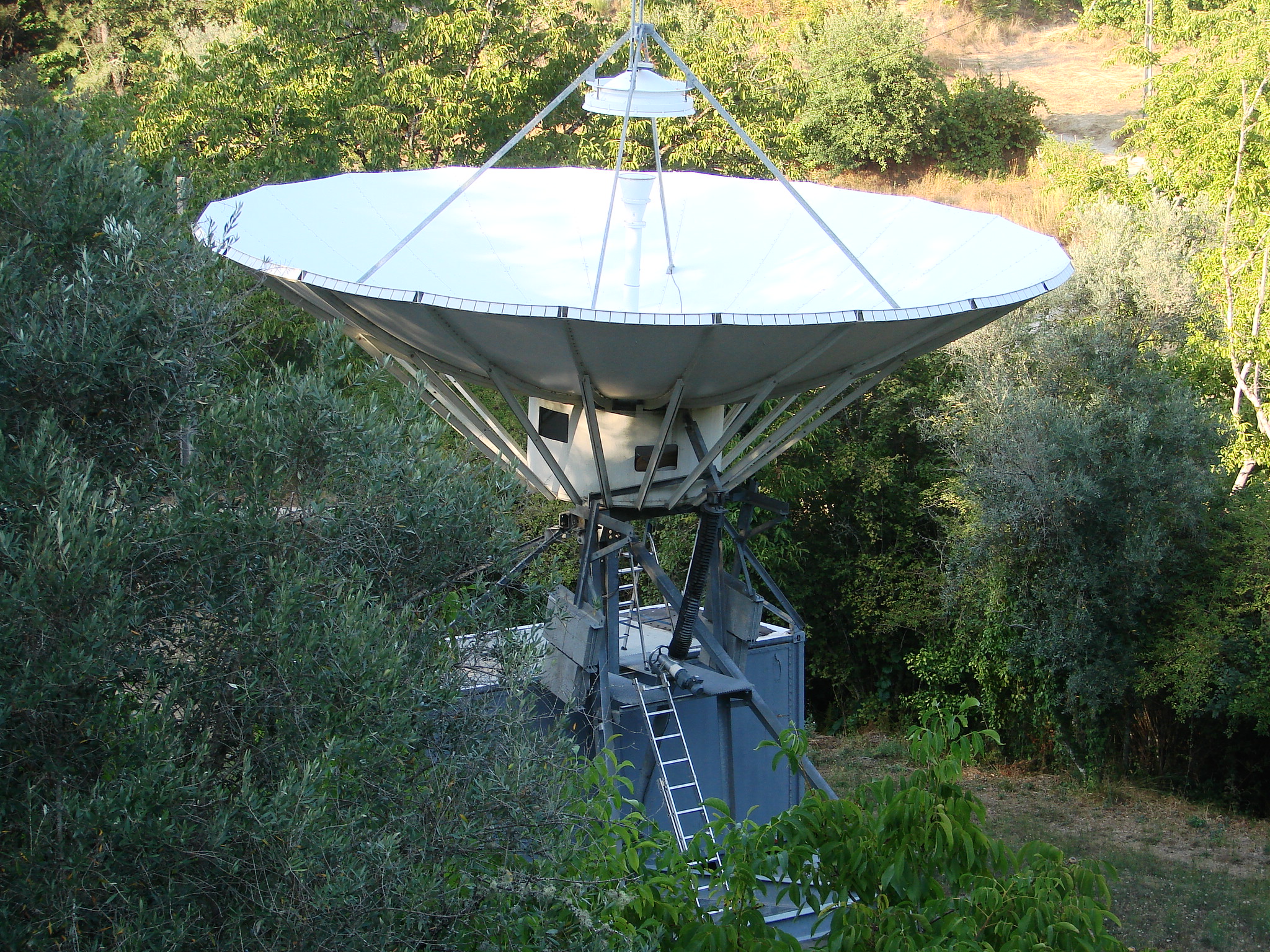
Fig.5 - Full horn

The resulting edges are much steeper because frequency jittering is less.

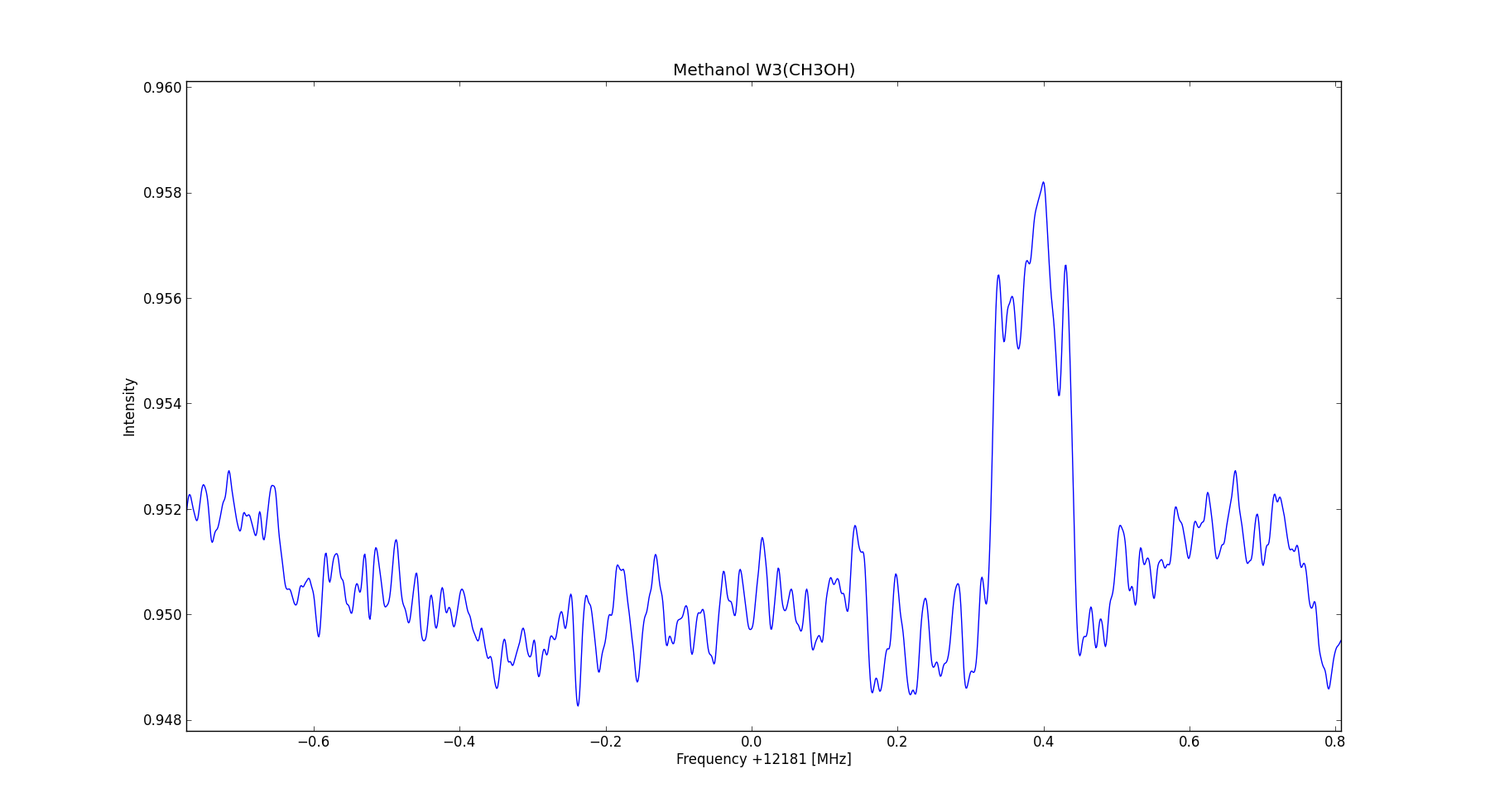
Fig.6- Steep edges

Now, back in the nl, we have analyzed the measurements some more.
In Portugal, we made a run with a bandwidth of 1.024MHz, so we could expect more frequency and km/s resolution.
Funny to catch a wave, swaying around by the doppler effect, but pointed exactly to by the calculated sky frequency.
I calculated the sky freq with my own script, but there also are sites like http://neutronstar.joataman.net/technical/radial_vel_calc.html to do that for you.


As I said earlier; still there is this strange amplitude variation and slow frequency shift over time as can be seen in fig 7.

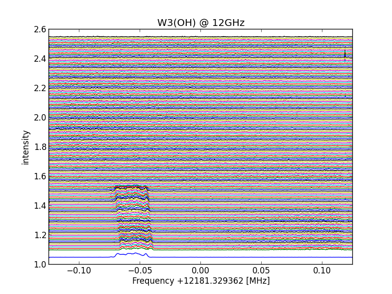
Fig.7- All lines

We compensated that again by bin shifting each 5 minute cfrad result as function of time, and only then they were added/averaged.

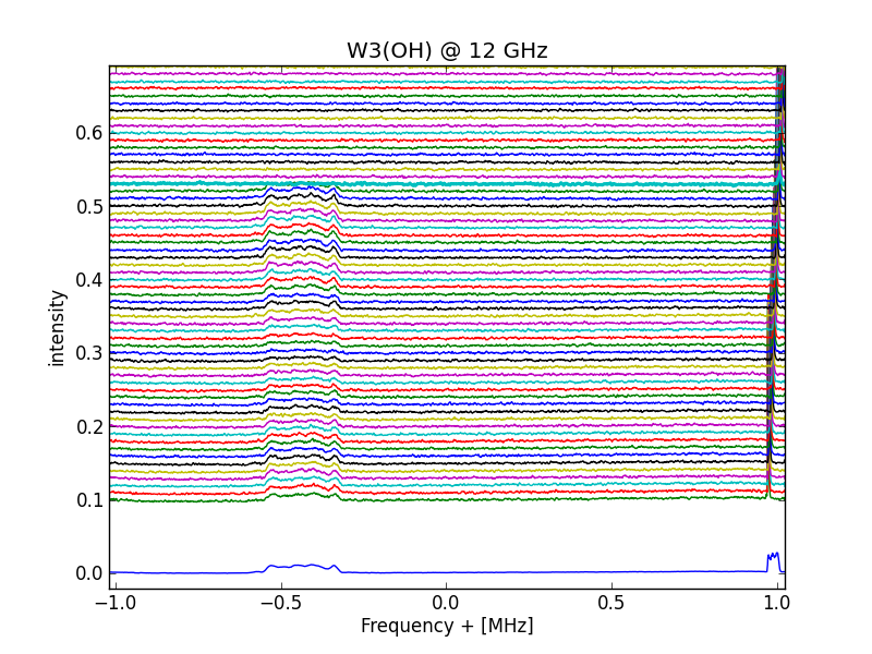
Fig.8- All lines shift corrected

Fig.9- Sum of lines

W3(OH) is a star forming region; this means that a gas disk is rotating around the center where a star can be born.
Over several years time it has bee noted that the gas masers move outward. This implicates that they are forced to do so, because in principle they move inward to form the star.

This gives the indication that the star has ignited, and expelling solar wind, which moves the gas ring close by outward, and clearing the nearest parts of the disk by that wind and uv light so the disk becomes a torus.


Still, the star cannot be seen on a visual picture.see http://simbad.u-strasbg.fr/simbad/sim-id?Ident=W3(OH)

Fig.10- No optical W3(OH)

It even does not have a filled WIKI page; so unpopular are non optical things.

Although the SGRT beam is 0.15 deg, the masers cannot be resolved of course; we are looking at a solar system XXL size.
But that problem the radio astronomers also had in the past.
They tried to separate the peaks by assuming Gaussian sources.


Later with VLBI, better 'pictures' could be made, and separate local maser regions (dots) could be seen.

Fig.11- W3(OH) contour with maser dots

As an amateur association we still lack that luxury, or cooperation to make a VLBI, so I tried to separate the peaks with calculations.
First we tried excel. Below you see how the resolver function can adjust the Gauss curves in frequency, peak hight and peak width, so summed all together gives you the original curve.
The problem is how many sources are there hiding in the result. I tried to estimate that by differentiating the curve twice. In this way all the bends in the curve show as peaks, trying to hide their existence.
In total I counted about 20 gaussians above noise level. This number was taken as a starting parameter for the solution.
Another initial seeding which has to be made is the size of the cloud, or the width of the Gaussian.
I took the size of the smallest peak as a standard; reasoning that the turbulence in the disk/torus was the same everywhere.

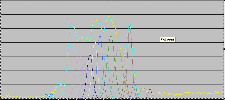
Fig.12- Gaussian

So,the Gaussian curves in the final solver run represent the individual masers, and when they are added gives you the curve you actually received with your dish.

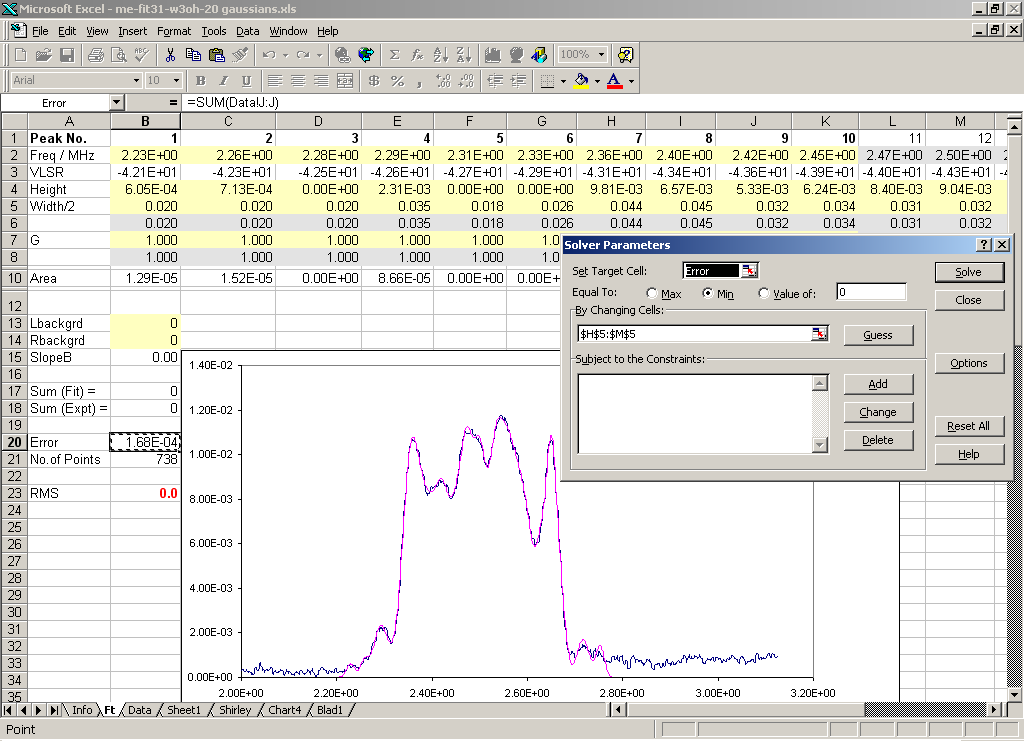
Fig.13- Gaussian fit excel

We now can compare this to papers in which VLBI astronomers have identified about 50 individual masers.
I omitted all the weak masers from that list and just took the 20 strongest. The result is very satisfactory.
In the picture I have connected some of the gaussians with the W3(OH) locations where they come from.

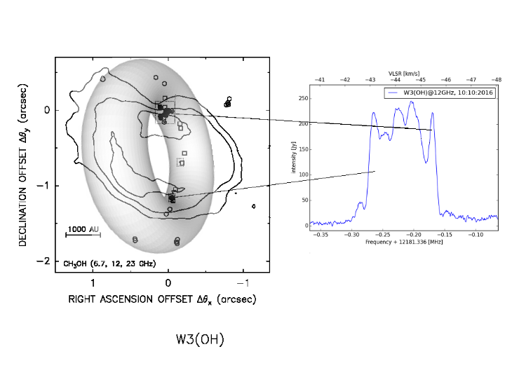
Fig.14- Torus projection and the Gaussian sources

You can deduct that the torus is rotating counter clockwise.
Accurate VLBI measurement shows that at the left part of the torus no masing can be seen.
So you can also deduct that we must be looking at the bottom side of the counter clockwise rotating torus.
It is more clear for me now why the front side of the torus does not emit maser signals.
Masing is obscured/attenuated by the thick part of the ring towards us.
So the masing is coming mainly from the inner part of the ring illuminated by the star.

To make things more complicated; there also seems to be a 'champagne' flow of gas from the poles.
Where does that material go; does it return in a high ecliptic orbit. Can we see that also in our solar system.

Some FAQ's;

As I said in other projects; each line is the result of 5 minutes of integration (100000 spectra averaged) with an efficiency depending on sample rate.


While measuring I moved the dish up and down, left/right increments of 0.01 degree to find the maximum signal.
I do that by monitoring one of the ten sub bands of the 5 minute FFT result. In the stacked graph fig 7 and 8, you can see that the amplitude of the source changes because of my optimal pointing trials.
The dongle is set to the AGC mode.
That also means that when the monitored track goes up, the others go down.


The measurement stopped, simply, because there were a sufficient number of 5 minute lines/results, so I gave the system instruction to go to the park position and put the clamps on, but I did not stop the capturing.

In the zip files I added all the referenced papers href="http://www.parac.eu/w3(oh) papers.zip"> here in a zip file.

Michiel Klaassen november 2016



From 2016, I have been measuring the maser W3(OH) at 12GHz every year. The 20>3-1E transition gives a photon on 12 178 595 000 Hz.
It appears that it is not easy to repeat those measurements every year when you change the feed and equipment all the time.
The problems are the pointing accuracy, the thermal drift receiver chain and the frequency accuracy.
But we do our best.
So when measuring W3(OH) I wondered if the curve form would change in my lifetime.
I have read that the water masers last about 10000 years and then they disappear. The circumstances have to be just right for masers to operate when protostar evolves from rotating clouds to star ignition.
At the end of life, the star starts the production of the lighter elements, and then the combination of the elements into molecules can happen, and again masers are formed and can stimulate radiation.
I have no idea if the next reasoning is correct, but given the lifetime of a star to be e10 yr and with our eyes we can see about 5000 local stars, the number of 'maser stars' could be 0.5.
So, not many maser stars can be seen with our amateur radio eyes.
Here is the graph of the maser light curve of W(OH) @12GHz.

W3(OH)-2016-2017-2018-2019

There are some differences in time, but not so large that it is obvious; differences are within the noise pp-level.
At Vlsr -45.2 the intensity seems to decrease in 2018 and 2019, as is the feature at -44km/s and at -43.2 in 2019. The feature at -43 seems to vary every year.
You would expect that the clouds circling to protostar will rotate faster when they move closer to the protostar, and so the rotation velocity will increase. This will result in the received signal to show a increased frequency shift with respect to the central system velocity.
The problem is that with a single telescope the beam is so large, that you cannot single out one origin of a complex star system; you need a very large telescope interferometer to do that.
It also appears that the masers are just spots in the star system; on a place where the circumstances are just right.
After the masers where discovered some observatories started programs to monitor them on a regular basis.
One of them was with the Medicina telescope in Italy. Here also is a W3(OH) graph from that data of the water molecule on 22GHz.

W3(OH)-27mar1987-22feb2007-22GHz

I plotted the logarithmic of the intensity axis, so the curves would not overlap; so that you can see the shift of the velocities more easy. (bottom is old)
On the Medicina graph I also noticed that there are more weak bumps; like on 30km/s. On the 12GHz graph, you can also see two bumps on -29 and -31km/s on the 2018 graph.
To try to find trends, I connected likely the same bumps together. You will see clouds appearing, drifting somewhat, and then disappearing again.

W3(OH)-27mar1987-22feb2007-22GHz-trend

w3oh.tar.gz: Download the original Medicina Radio Telescope data files