[HOME]   [WEB ALBUMS]   [PROJECTS]   [ARCHIVE]   [DOWNLOADS]   [LINKS]  



PROJECTS



project MK19: Measurements on the galactic anti-center

During a test session in the Dwingeloo Telescope (DT), we tried to measure the anti-center of our galaxy.

The reason for this is as follows. There are two directions where the galactic hydrogen gas as seen from our location in the galactic plane is not moving relative to us or moving away from us. The directions are to the galactic center and to the anti-center. In all other directions along the galactic rim the gas moves with speeds up to hundreds of kilometers per second relative to the sun or away from it.

In order to detect minimal movement in the gas, the best directions are L=0, b=0 or L=180, b=0. Here we can determine whether the gas is moving in other directions, such as a rolling movement along the length of the arm, like a sausage can rotate along its longitudinal axis. If this is so, then the upper part of the rim moves toward us, and therefore the lower rim away from us, or vice versa.

Unfortunately our third measuring session yielded only 1 usable profile, so for more profiles a lot of hours more would be needed. It is also a problem that the coming months the DT will go into revision and is no longer available for measurements. However, it appeared that the DT already performed the needed measurements and these are available to everyone on the net via the following link; http://www.astro.uni-bonn.de/hisurvey/profile/

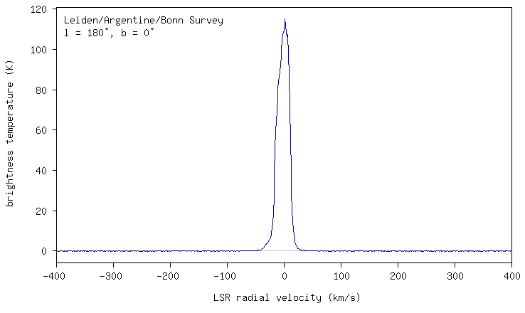
Fig.1 - Typical profile.

This allows everyone with an internet connection to download a hydrogen profile for each degree on the sky. The frequency axis is converted to the range -400 to 400 km/s, and the resolution is 1.3 km/s. The intensity is given in degrees K, but the negative values can be seen as signal noise. Furthermore, the (sub) area under the curve is a measure of the gas density. A negative speed means that the gas in coming toward us, and a positive value means that the cloud is receidung us.

For a first overview of the target, we take the range L = 160 to L = 200 at b = 0, and we get 40 profiles that we copy into Excel and / or Python. Note that points or commas in your Excel version are interpreted correctly, otherwise you have to use an editor to convert it. This gives the following graph.

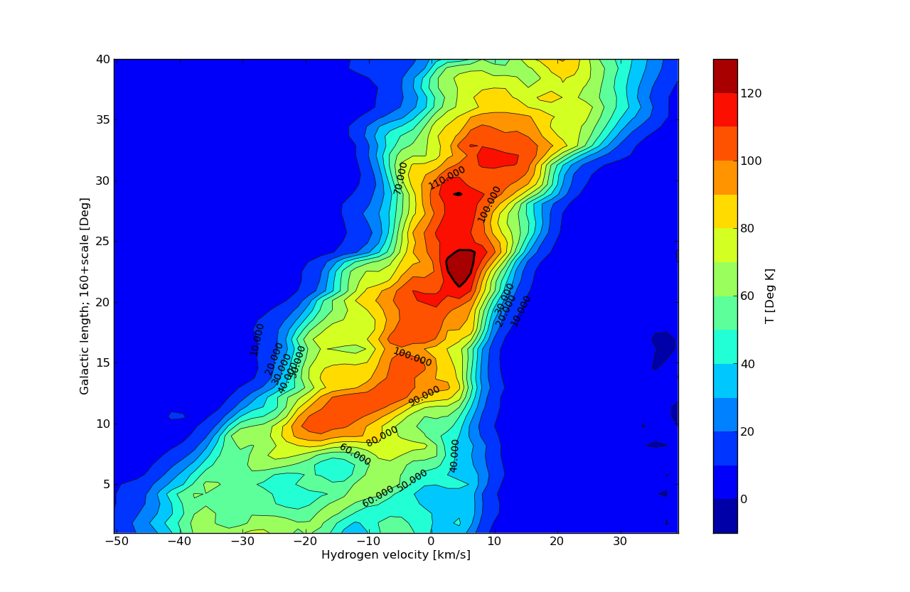
Fig.2 - Galactic Anti Center Overview.

First notice that when b = 0 the signal is maximum at L = 183 and 5.2 km/s, and not at 180 and 0 km/s. We also see that the signals from the moving gas clouds clump together in this section, the red / dark red area. When we going forward or backward in the longitudinal direction, then the spectrum becomes wider, because the clouds come to us or moving away from us.

First measuring method We examine the cross section, starting with L = 180 degrees. We download 80 profiles from b = +40 to -40 degrees. One can also do it yourself, for example on b = -38, one can find an anomaly, but here we show only the portion of b = b = +10 to -10 degrees for our research.

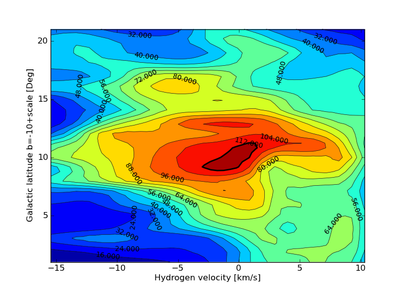
Fig.3 - Anti Center Detail.

We see the following, on the horizontal line b = 0 and the signal broadening but still not reduced to zero , the movements of the arm and arm behind it still causes a speed variation from -15 to +10 km / s. Next we see on the vertical line in the middle that the part above the middle bends towards the left side and below the center to the right. This means that the upper part comes toward us, and the lower part moves away. Right in the middle we see the opposite, the dark spot goes from bottom to top from left to right. This means that the gas above the zero line moves away from us and below the zero line gas comes toward us.



Second measuring method We can also measure the roll by subtracting the profile of b = -5 of that of b = +5. If there is no movement of the gas, then the difference between the two profiles is 0. If this is not the case, then a small frequency/velocity shift of the two profiles, will give a result which has the shape of a sine or a minus sine wave. By measuring on successive latitudes of b, and subtract the pairs of b, we can see the roll rotation speed dependant of b. This gives the following result.

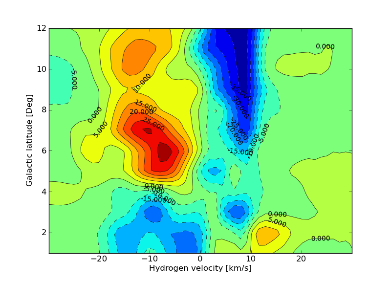
Fig.4 - subtracted profiles.

The red part is the plus intensity and the blue area the minus intensity. We can see the typical cosine form with b smaller then 4 degrees and the sine form at b > 4 degrees. The speeds at b> 4 degrees is about 10 km/s approaching above the galactic plane and 10km/s receiding below the galactic plane.

Measuring method 3 The third method to interpret the measurements is to use the radial rotation in order make the shift visible. As said before, we had expected that the zero line of approaching gas and receiding gas should be on the line L=180 and b=90 to b=-90, but this is not the case. What we can do now is find out where the zero line is running in reality. We look at a fixed latitude b and then we vary L, and look where equal amount of gas approaches us as is receiding us. If these values are equal, then we denote the galactic longitude where this happened. Example We begin with b=0 and vary L between 160 and 200 degrees. All these profiles are stored in excel. We add all intensities for each profile of the approaching gas. Similarly, for all intensities for receiding gas. For each profile, we get three values, sum of the approaching intensity, receiding intensity and total intensity. We do this for all profiles and make a graph.

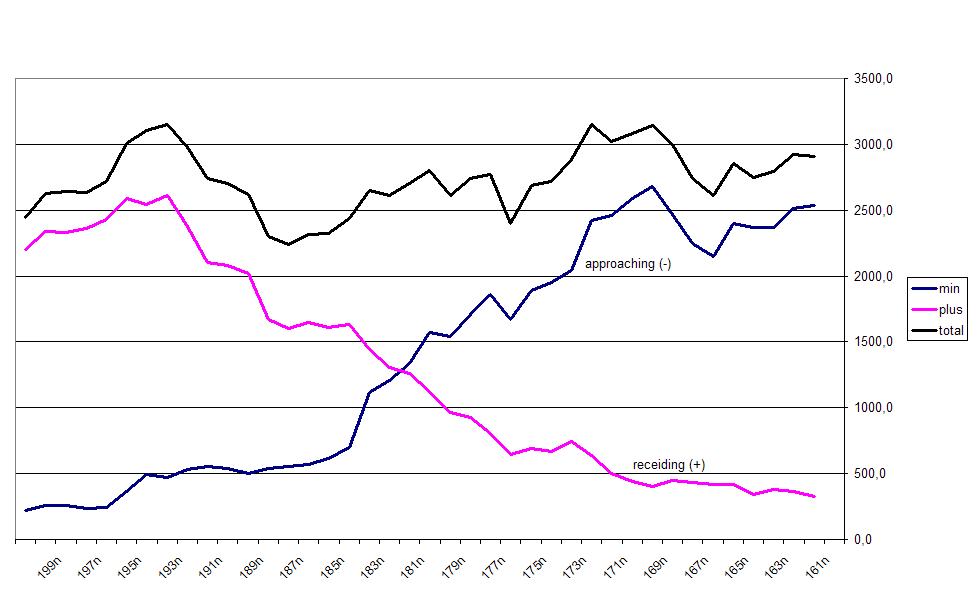Fig.5 - Zero Velocity Point.

We see now a crossing where equal amount of gas is approaching and receiding us. For b = 0 this point is at 181.4 degrees. We do this now for all other lattitudes of b; from b = +12 to -12 degrees. Thus we get the following zero-line graph.

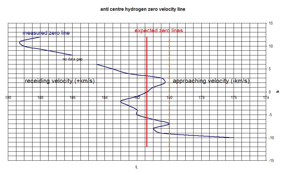Fig.6 - Zero Velocity Line.

Now how can we explain these facts. At L=181.4 degrees and b> 0 is the gas is still approaching us and at b smaller then 0 it is still receiding us. This additional movement is not caused by the radial rotation, but by a latitude rotation or roll. The conclusion is, therefore, that the arm rotates around its axis, such as a sausage in its longitudinal direction. The rotation is very small and has a speed many times smaller than the radial speed of 200km/s. The roll rotation is about 5 to 10 km/s at a height b of plus or minus 10 degrees. Outside this angle we see some increase in speed until the speed decreases when b> 12 degrees. That gas is no longer participating in the roll rotation. Remains the region between b = +4 and -4 degrees. Here we see a reverse speed. What is striking is that the speed variation per angle is equal to the above measurement, but reversed in direction. This can be explained by the idea that we are observing the next galaxy arm, (through the center of the nearer one), which rotates in the opposite direction. To explain this more, see accompanying figure.

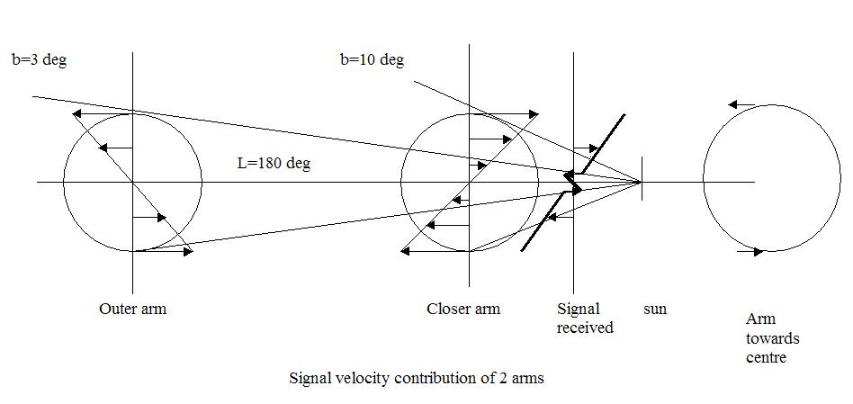Fig.7 - Rolling Arms.

In the figure we see that the maximum receiding rotation of the outer arm edge at an angle of about b = 4 degrees. Similarly, at b=-4 degrees the gas is approaching us. Note that the compensation effect by the radial speed is shown relative to the zero line measurement so it is displayed in reverse. If we assume that the nearer arm diameter and is the same as the outer arm, then it is in agreement with the observations. So, our immediate neighbour top arm turns to us, and the outer arm top away from us, at a speed of approximately 5 to 10km/s.

If we make the same scan in the direction of the center L=0, b=+12 to b=-15, then we get the following graph

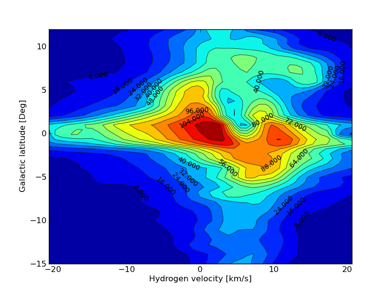Fig.7 - Galaxy Center.

Here also we see that the gas is coming to us at b=+5 and the gas is receiding us at b=-5 degrees. So the roll direction is the same. It looks like we are in a downstream between two galaxy arms.

Andromeda Now there seems reason to believe that not just our galaxy exhibits an arm roll rotation, but this could also be the case for all galaxies. A test would be, to look at the nearest galaxy Andromeda, to investigate this effect. To measure this, we have to do a measurement over the neutral velocity axis of the galaxy, so on the line separating the approaching gas, and receiding gas (with reference the center). Instead of a straight sharp dividing line, one would observe a small wavy line. The differences in speed between the center of the arms must then be measured, and they have to be opposite to the center of the next pair of arms. It will be difficult to do this with the DT to detect, but perhaps it is possible with cooperation of other radio telescopes when using interferometry to improve resolution.

In short, the DT measurements still give us many hours of discovery fun, while in this report we only used 2% of the available measurements.

Michiel Klaassen 29-04-2012