[HOME]   [WEB ALBUMS]   [PROJECTS]   [ARCHIVE]   [DOWNLOADS]   [LINKS]  



PROJECTS



Pulsar detection with an oil drum antenna

Introduction.


Part of this text was also used for the The American Radio Relay League (ARRL) book.


Urban area's are more and more polluted by Radio Frequency Interference (RFI). Of course we benefit from the 4G, 5G, local hot spots, wifi and wifi extenders, remote metering, remote control toys etc. Although there is strict regulation on the used frequency bands,the signals can be so strong that they saturate sensitive radio's.
Astronomical signals are very weak, and mostly only can be detected when thousands of the same signals are stacked, the same way as done with optical astronomy.
An advantage is that the radio waves come from above and not sideways. So to isolate the unwanted RFI in the first place, an antenna for radio astronomy has to be extreme directional. A yagi is not, because the active element can be seen by RFI from the side and even from the back. So, how to choose the right antenna.


1. Antenna hardware setup
We have to use a horn antenna with the active element hidden deep into the base of the horn. Pulsar signals are strongest on lower frequency's like 400MHz. That implies that the horn dimensions must be large. When we use the horn calculator from http://parac.eu/downloads.htm then it gives us the dimensions like of an oil drum. A second hand oil drum is cheap, so we can use that. To scoop as much of the 'radio rain' as possible a large 2m wide flare is added.
see figure 1.

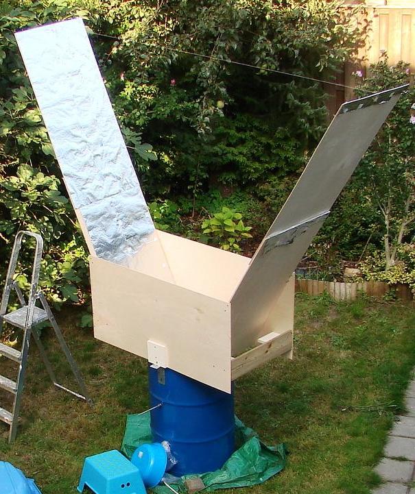
Fig.1 - Drum horn proof of concept

We used an oil drum 35hX23d inch with aluminum foil covered plywood 240x60cm. Sides removed for clarity. freq 460MHz. Probe 15cm long, 22cm from bottom. According to Huygens law the beam width now becomes 67X20 deg. We just can let the pulsar drift along the wide angle of the beam.
Connected to the N-connector of the probe we have a broadband LNA; 25dB, simple 75 Ohm cable, a power inserter and then a cooled Nooelec SDR.

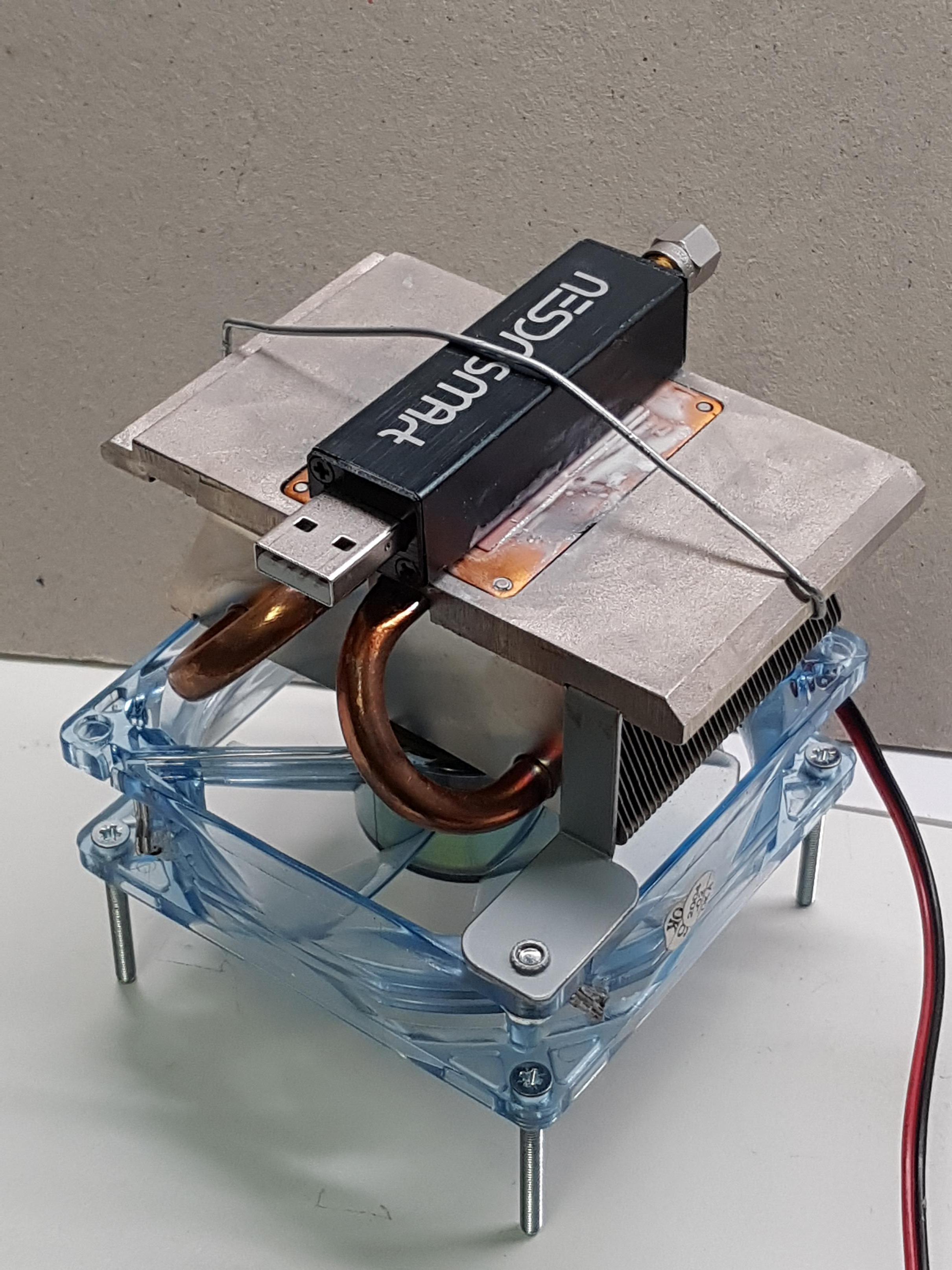
Fig.2 - Dongle on heat sink with fan

Cooling is advised to ensure a stable sample rate, because of a stable x-tal frequency.


2. Capturing the pulsar.
Download the rtl_sdr.exe tools from internet or parac.eu downloads page.
The command can be;
start /realtime rtl_sdr,exe -s 2e6 -f 459e6 session1.bin.
where "start /realtime" ensures that the execution is performed with the highest priority.
-s 2e6 is sample rate = 2000000Sps.
-f 459e6 is frequency set to 459MHz.
session1.bin is an I/Q file name written to disk.
You could add a number for the samples to be recorded, but this can only be for a short time period. A general method is to omit the - n command and kill the recording after 0.5 or 1 hour.


3. Post processing the raw data.
3.1 First use the Pulsar Period Calculator 2PC; the for Windows automated TEMPO tool. It can be downloaded from http://parac.eu/projectmk17c.htm.
Important actions for determining the Tempo pulsar period time are:
-Note the exact moment of observation; date and decimal time in UT.
Like when observing a passing train sounding its horn, the tone will not change much when the train is far away.
When however the train passes close by, the change in tone is large. This is the same with pulsars observed from the rotating planet earth.
-Note the exact location of the observatory in latitude and longitude.
Fill in the other variables and run the app.


3.2 Use 3PT, the 'Pulsar Post Processing Tool'; it can be downloaded from http://parac.eu/projectmk17b.htm
The first part (3PT-calc) processes the IQ data string. Dependent on the amount of BIN's the user want to see, the bandpass corrected period chunk is divided into bin parts.
Each BIN chunk is FFT and split into 20 frequency channels and a sum file, and written to disk. So each written file represents one pulsar period.


3.3
The second part (3PT-plot) can read all period files required. Next it can ignore one or more periods or one or more frequency channels when they appear to be invested with RFI.
For judging the quality of the data captured a graph of the bandpass curve is given. It has to be smooth without too much large spikes. Next the bandpass curve for 20 frequency sections is shown, together with the used band correction curve which is used.
Next the RF intensity over time is shown. The curve has to be flat over time. The SDR must not become hot; this will decrease the gain or signal strength, and alter the Xtal frequency drift. The shifting radio frequency is not a problem for pulsars, but the sample rate derived from the crystal will vary.
The product of sample rate and period time is constant when the optimal S/N is found. So, if it is known that the pulsar period time is exact, then the sample rate error can be determined and vice versa. see also http://parac.eu/projectmk17c.htm.
We run the total captured period for the first time.

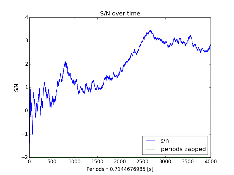
Fig.3 - Signal to Noise full range

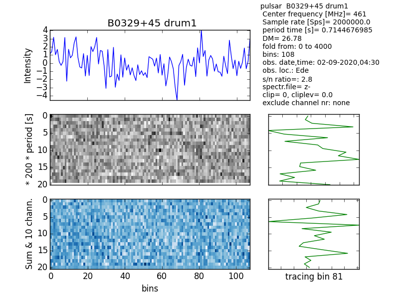
Fig.4 -Multiplot B0329+54 full period range

Often in the graph of the S/N we noticed that in the first part the S/N value varies, but then starts to climb and next flattens.
So for the second run we enter the S/N rise starting period and the flatten period endpoint.
The climbing increase of the S/N value is a good indication of presence of a pulsar. A wavy variation could be caused by passing clouds or tracking variations. If the standard deviation of a period is large, then this period is rejected or 'zapped'.
Also the pulsar period time can be adjusted, and not to be taken at the start, but on the moment the S/N rises.
When this new UT time is entered, the 2PC tool gives a new period time and recalculation with 3PT-calc should give a better S/N ratio.

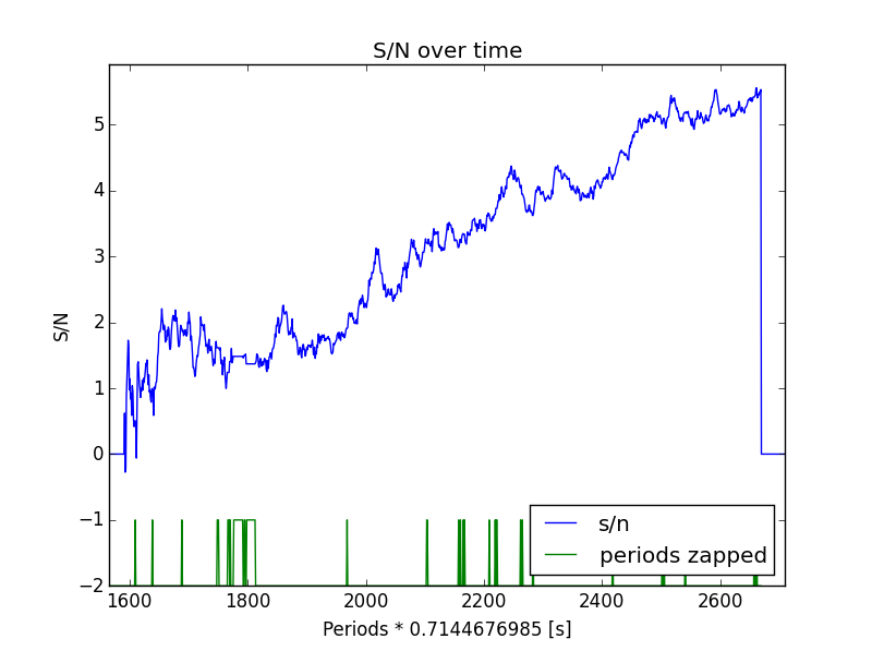
Fig.5 - Signal to noise selected range

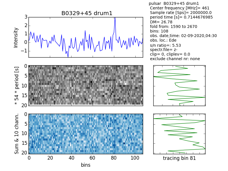
Fig.6 - Multiplot B0329+54 drum1 selected range

See other results here; http://parac.eu/projectmk17b.htm


5. Audio. When the pulsar result shows a peak above S/N level of about 3 then it also can be made audible.
Download the audio tool from http://parac.eu/projectmk17d.htm
Results can be found here:


https://www.youtube.com/channel/UCFB8N_2WmA3mxc4i8KN2T_A.
So if you dare; start the drum session, and next fast forward it to save lifetime.
If you have time, you will see that the amplitude of the stacked result is lowering (as expected) and the single pulse period amplitude stays the same. The squelch level is set to 0.6 times the peak value, but you can change that in the Ap.cfg file.
I added some pictures of the details of the setup along the way to make this presentation less boring.

For general information and fine tuning see the full section of http://parac.eu/projectmk17.htm.

See also the article, in cooperation with Peter East, in the 2020_oct SARA journal.






Michiel Klaassen october 2022