[HOME]   [WEB ALBUMS]   [PROJECTS]   [ARCHIVE]   [DOWNLOADS]   [LINKS]  



Pulsar folding with sound

To explain to my girlfriend and our children some more about pulsars, I decided to take our captured data and add a visual and audio interpretation of the pulsar.
From the period data 100 to 545 (fig1) we took the short range 100 to 200 periods; fig 2.

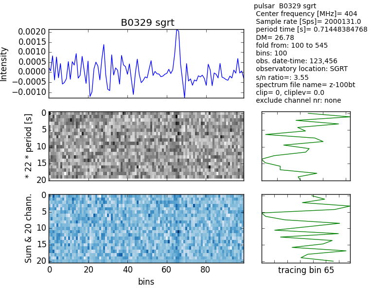
Fig.1 - Multiplot-100-545.

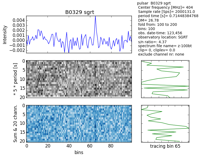
Fig.2 - Multiplot-100-200.

Next we selected periods 100 to 200 of the datastream and folded/added it in real time every period. You can see in the video that the pulse is rising from the noise. At thesame time the peak above a certain level will generate a tone. This tone can also be so low in frequency that it gives the 'thumb' sound of a pulsar. The background sound can be set to a loud noise sound level or it can be set to attenuate completely.
The total presentation time is 100 periods of the B0329+54 pulsar, so about a minute.


Configuration is done with the Ap.cfg file; it contains the following:


0.------pulsar audio folding------------
1.pulsar name = B0329 SGRT
2.pulsar period time [s]=0.71463071463
3.spectrum file name without extension=z-100bt
4.fold period from =105
5.fold period to =200
6.audio pulse squelch level (0..1)=0.998
7.audio noise volume (0..1)=0.1
8.graph select (0:off, 1 or 2 or 3(both))=1

On item nr 8;
Select 1 to see only the stacked pulsar profile.
Select 2 to see only each period profile.
Select 3 to see both.
If the pulsar is fast; like Vela, Then the graphs give too much delay. You can turn the graphs off by selecting "0", and only hear the audio.The final result graphs will show at the end


The tones were generated with an online tool from
https://www.audiocheck.net/audiofrequencysignalgenerator_sinetone.php
Also we ripped sound from a youtube track with Audacity.

We used the python pygame modules to handle the sounds. To run the python script yourself you need pygame installed; see
https://www.pygame.org/download.shtml


More specific info:
The data captured in this session had a lot of RFI (Radio Frequency Interference ). Later we could trace that back to the LAN (Local Area Network) cables.
The source period files or spectrum files were generated by the 3pt-calc.exe program. Each file consists of a number of spectra for each bin range and one sum spectrum bin range. The sum of the spectra is also available in the sum bins (nr 10 or nr 20). The latest 3pt calc program splits the spectrum from 10 into 20 parts.
This audio script is loading the successive period files and scans the bins for the maximum value. Next it scans again to flag every bin with an amplitude higher than the squelch level. This flagged bin will generate an audio tone.
In the right side monitor window of 'spider' you can see info of each period.
The first value is the period number (from 100 to 200).
The second value is the bin number of the maximum found amplitude. In the beginning the bin numbers vay, but later, from period 130, the bin number is the stable number 65.
The third value is the period time of the audio period.
The horizontal line is the squelch level; noise can be heard when the amplitude rises above this level.

The video can be seen here
pulsar-folding-and-sound 1.mp4  


A second video shows thesame folding, but now the individual periods are also shown in red.
The amplitude of the individual period is actually 4 times larger, but in the graph reduced for clearity.
pulsar-folding-and-sound 2.mp4  



We could bring down the size of the Windows executable from 1GB to 35MB.
A method was found here;


https://sites.google.com/site/rangsiman1993/programming/python-reduce-size-of-exe-pyinstaller-on-conda?authuser=0

"""
Step-by-Step method by Rangsiman Ketkaew:

1. Create new conda environment:
conda create -n NAME_OF_NEW_ENV

2. Install pip using conda:
conda install pip

3. Install other packages that your application requires using pip, for example:
pip install numpy
pip install matplotlib

4. Use conda or pip to show all packages installed in environment:
conda list
or
pip list

5. Install PyInstaller using pip
pip install pyinstaller

6. Now you are ready to make executable file from Python source code using PyInstaller:
pyinstaller example.py --onefile
"""
After closure; re-enter your virtual environment by 'conda activate NAME'

Together with the period files generated by 3pt.exe, the Ap.cfg, and the .wav files, etc; are compressed in a zip file here  
To use it; unzip in a folder and run pa22.exe.
A window shows information, and while running, the period number, the bin number, and the period time are displayed.
Via the config file Ap.cfg other parameters can be set.
This version of the program pa22.exe runs ok in Windows-10 64 bit.



Michiel Klaassen January 2022






Vela pulsar fold and sound with Matplot blitting
Yes; Blitting is the word.
I found old IQ data I received from Guillermo Gancio. He captured the vela pulsar with the huge 30m telescope of the IAR in Argentine.
https://en.wikipedia.org/wiki/Argentine_Institute_of_Radio_Astronomy

This pulsar has a period time of only 0.09 seconds. The standard plotting software I had could not keep up displaying the graphs, so I had to change things.
So I discovered Matplotlib blitting. That is plotting only the necesary variing things in a plot.
With this method you can increase the display rate from 5 fps to 120fps.
On the inet there are lots of Python blit, and animate examples; mostly very complex and hard to understand. A lot of Classes, .self and Defines are used; too complex for me.
So, once again, in the end, I discovered the essence and bundled it all into an exe.

With this version I added the option to zap (discard) a period of data. The decision is made by calculating the standard deviation (std) of that period.
If is is engulfed in strong RFI, then the std level will be high. The decision level can be set via the config file.
While running the program, the std level is also printed onto the plot, so you can set the zap level just above that plot level.

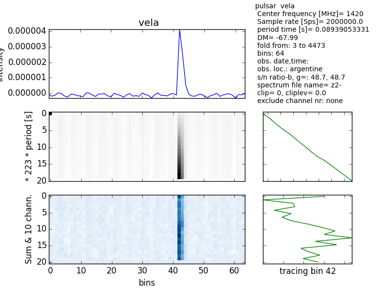
Fig.3 - Multiplot-Vela.

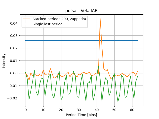
Fig.4 - Pulsar profile Vela.

The blue line is again the squelch level, above which a sound is generated.
Because the plot speed is higher now, there is no need to gain speed by de-selecting one of the two graphs.

A peculiarity is that the data contains a very strong hum of about 150Hz. Perhaps it is a 50Hz overtone or a control signal sneaking into the data stream, but as you can see; when averaging the data the pulsar profile can still be extracted.


Another peculiarity is that the pass band curve displays extra bumps. Because the capturing was done on 1420MHz these curves come from neutral hydrogen.

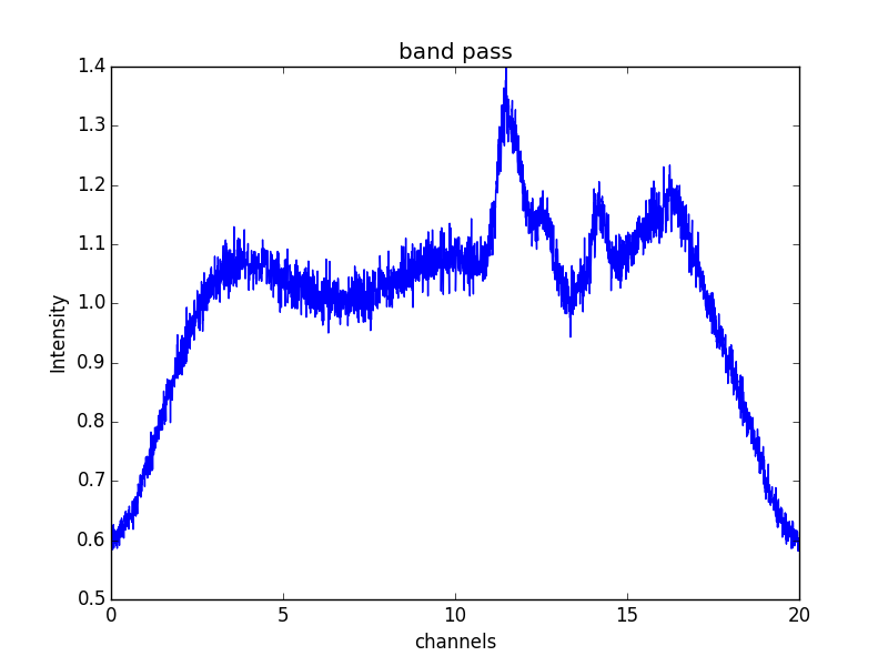
Fig.5 - Band pass Vela plus H1.

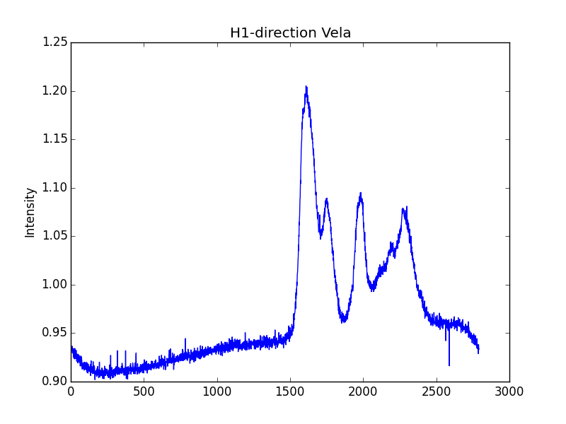
Fig.6 - H1 direction Vela.

To verify this signal we can look into 'the' database of H1;
https://www.astro.uni-bonn.de/hisurvey/profile/
When we enter the RADEC direction of the Vela pulsar (08 35 20.65525 -45 10 35.1545), we get fig7. This graph looks exactly thesame.

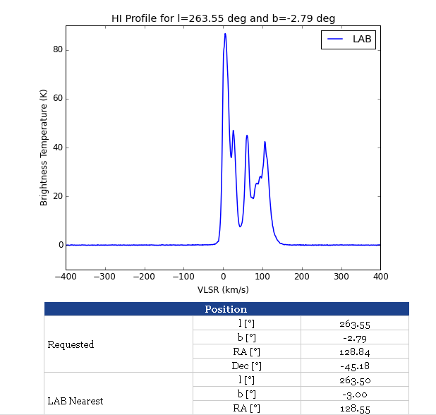
Fig.7 - H1 direction Vela.

Normally the curve you get in the frequency regime is mirrored. That is not the case here; so how is that possible.
Well, the frequency data was captured mirrored already, by mixing with a local oscillator signal above the frequency band of interrest. You can also note that because the DM is given as a negative value.

This new version of Pulsar Fold and Audio, incl VELA example data can be found on the website.here  


A video lasting 20 seconds can be found here
https://youtu.be/UBDJMebpwCA




Michiel Klaassen May 2022