[HOME]   [WEB ALBUMS]   [PROJECTS]   [ARCHIVE]   [DOWNLOADS]   [LINKS]  



PROJECTS



Pulsars; observations of pulsar B0329+54 with a RTL dongle

With the Sao Giao Radio Telescope we are going to capture pulsars also. However at the moment there is no time and also not the suitable feed to do so,. Also we do not have a 20MHz broadband receiver, no reference clock or oscillator and no precise tracking. All the shackles in the chain of receiving pulsars signals have to be right.

So to start this project, a better scenario is, to start with a big dish with a good feed, a good pre-amplifier and accurate tracking.
That is why we started by using the Dwingeloo 25m telescope and pointing it to the loudest pulsar; B0329+54; date and time; 13 january 2016 at 1900 local time.
The actual receiver was my own RTL dongle; see picture.

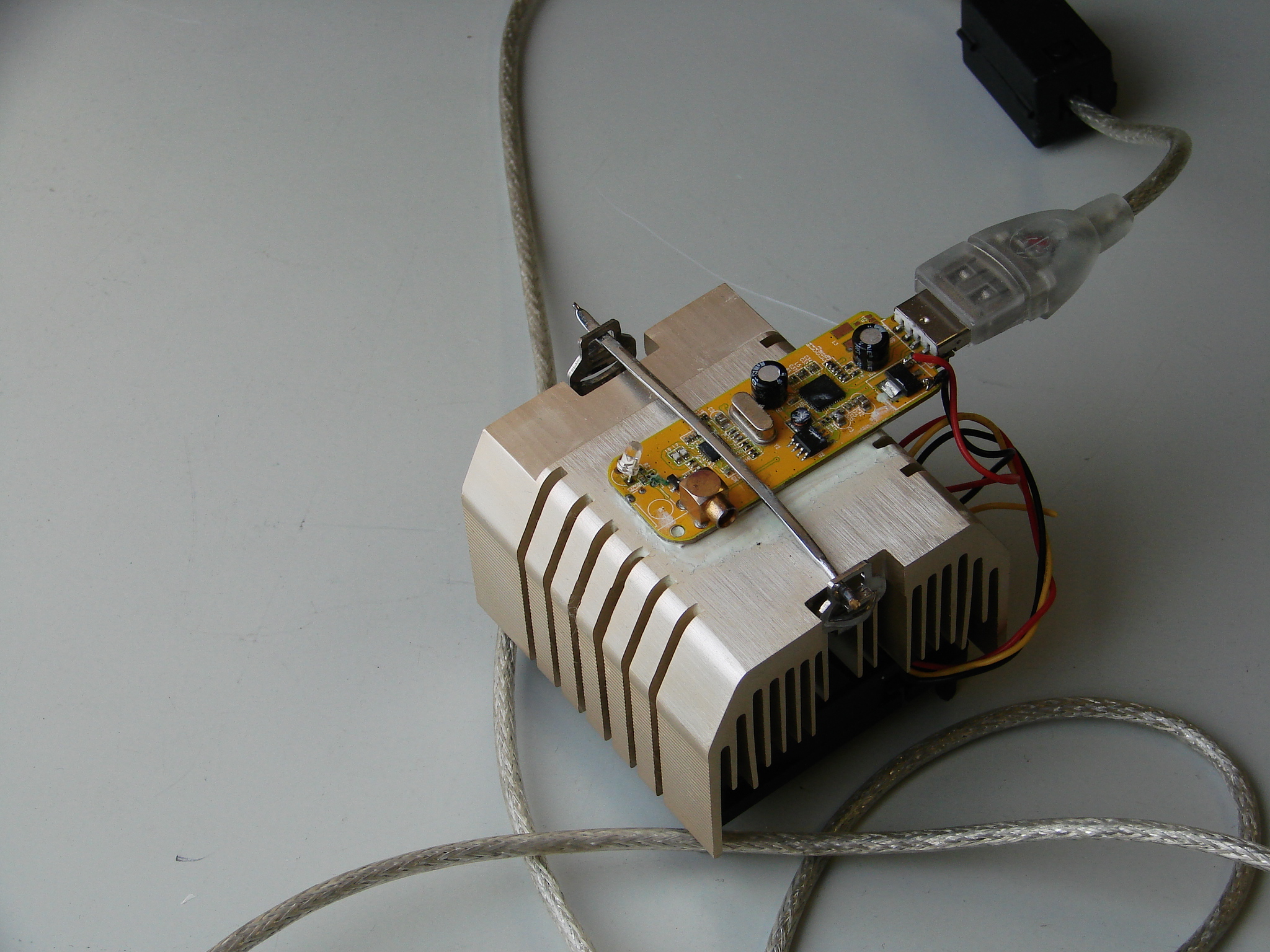
Fig.1 - Dongle on heatsink with fan

To keep it stable in temperature, the solder side is placed onto a heatsink. Of course that solder side is sanded flat carefully and thermal conductive pads and paste is used.

We did not have the illusion that we could hear the pulsar, so only an effort was made to capture the data and dump it onto disk. But first you have to find an empty region; free of RFI (Radio Frequency Interference).
This can be checked with SDR# and you can download it here or here.

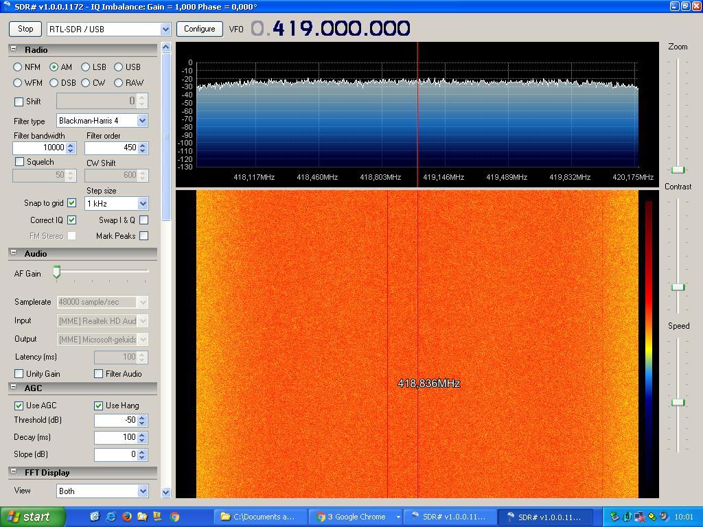
Fig.2 - Sharp screen example frequency setting

Remenber the frequency centre setting and the bandwidth, and close this utility.
The capturing software used was the well known rtl_sdr.exe; it can be found here, but also be downloaded here.

We could dump two files; one with a sample rate of 2MS/s here and one with 100kS/s here. During another run, the mechanics of the azimuth drive of the radio telescope had a problem and we had to stop the session.

The .bat files used for the 1st measurement was; rtl_sdr -s 2e6 -f 419.0e6 -n 2e8 dump2000a.bin, meaning;

-s 2e6; sample rate 2MS/s
-f 419.0e6; frequency 419MHz
-n 2e8; number of samples to process
dump2000a.bin; name of the file


With the pulsar period being 0.714s the number of periods measured will be 2e8/0.714/e6/2=70 periods (50 seconds). Note that every sample consists of two bytes; 1 "I" and 1 "Q" byte.

The second measurement started with the .bat file containing; rtl_sdr -s 0.1e6 -f 419.0e6 -n 1e8 dump100b.bin. This will give 2e8/0.714/0.1e6/2=700 periods, lasting about 8 minutes.



Next up; the task of analyzing the data. I made several scripts in python(xy)from here; it is like old "Basic" and fun to write. The first results given in fig.3; all the pulses captured in time.

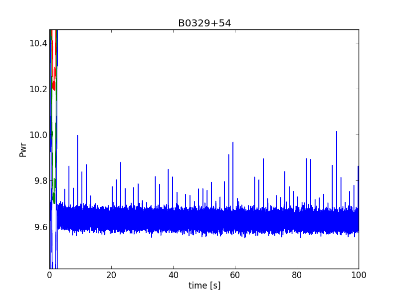
Fig.3 - received pulses, captured with 2MS/s, as a function of time

In the first few seconds the data is misformed, and the remarkable is that the following pulses are varying in amplitude. This variation is called scintillation; somewhat similar to the tinkling of the optical stars. However the radio scintillation is not caused by the earth atmosphere, but by the moving curtains of electrons in the milky way clouds.

We can zoom into a single pulse, and we note that the noise floor is not a flat line. We can improve that by averaging more pulses. The problem is that it has to be done in an exact rithm or period; the pulsar rotation period. If we cut and paste/stack every pulse with a shorter period time then we get this result.

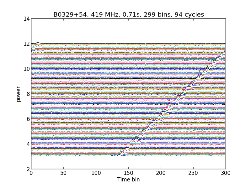
Fig.4 - received pulses, captured with 2MS/s, stacked with 0.71 second folding time

If you fold the pulses with a longer time slot, then you get the next result.

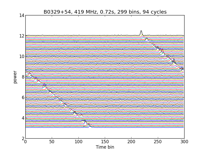
Fig.5 - received pulses, captured with 2MS/s, stacked with 0.72 second folding time

The best results you get with 0.714642471414 seconds folding time;

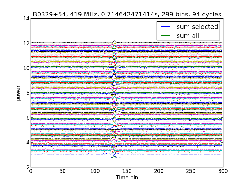
Fig.6 - pulses, stacked with 0.714642471414 seconds folding time

Now how can we find the optimal folding time. One way is to use TEMPO. This is a free utility; described here and can also be downloaded here.

A second way is to do a frequency analysis or FFT on the graph of fig.3.

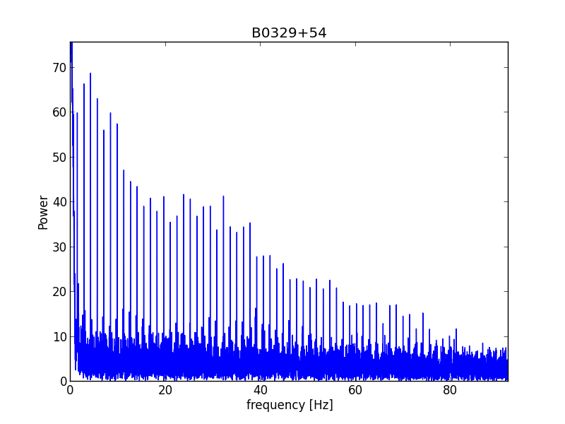
Fig.7 - FFT of pulse time line

Because it is a pulse form, you get higher harmonics. If we zoom in on the the 9th harmonic, the frequency is 12.5904Hz. The period is then; 1/12.5904Hz/9=0.7148303s. You could try to improve the accuracy by taking more harmonics.

Yet another way is to start from the estimated period time and scan for the best signal to noise ratio when the period is varied around the estimated value. This could give you a graph like this;

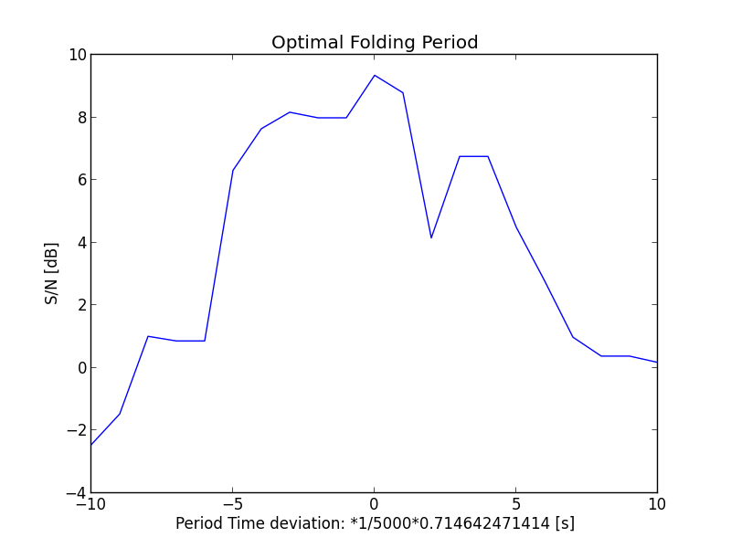
Fig.8 - Optimal folding period search

From fig.6 we can average all the folded periods. However a lot of periods do not hold a pulsar signal. If we take these also into the average, then the resulting pulse will be lower. Only the noise average will be better.
By selecting the periods with an actual pulsar signal we get the best result; see fig 9.
Selecting a window (boundaries for time, frequency or amplitude) is normal in pulsar analysis. See here

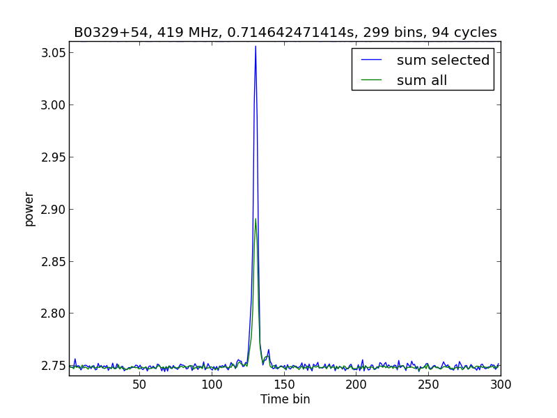
Fig.9 - Average all versus average selected

This is proof of the pulsar being detected. Later we can still further optimize the result, but for now we are shure that the pulsar period is correct. Now we can do an estimate of the diameter of the pulsar.
The rotation speed on the surface of the pulsar is v=ω*r. (1)
with ω; omega = rotations per second
v; speed in m/s
r; radius in m

Also ω=2*phi*f
with f; frequency=1/p we get:
ω=2*phi/p (2)
Where p = the pulsar rotation period in seconds.


Combining (1) and (2) we get:
r=v*p/(2*phi)

We know that the speed v cannot be higher then c: the velocity of light, so: v < c

We now have r<c*p/(2*phi)
With c=3e8 m/s, p=0.714 s, phi=3.1415, we get r<34e6 m.
So the diameter of the pulsar is smaller then 5.3 times the diameter of the earth.





To further analyse the data let us have a look at the spectrum. The data was captured with 2MS/s; that implies a bandwith of 2MHz, when the right calculation is done. As with the analyses of the hydrogen measurement in project MK6 you see that the bandwidth is not flat; it is bumpy and rolls off at the low and the high end. You can also note that the noise ripple amplitude on the low and high side is less than in the middle. That means that the amplification is less on that part of the bandpass. To make the bandwidth flat again you have to amplify the passband with a correction mask. This mask can be made by inverting the passband data. However that mask has got spikes ofcourse. To average these spikes, you can measure a lot of band pass masks and average them. Sometimes even that is not enough. The next solution is then to use a fitting polynome. When using a polynome there are no spikes anymore, and when multiplying the data with the passband correction mask you do not add noise.

So, now you have a flat passband result, and you can split them. In the first attempt I split them in ten channels; 0-200kHz. When plotting it looks like this:

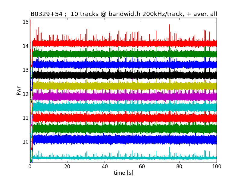
Fig.10 - splitting into 200kHz channels

Zooming in you see this:

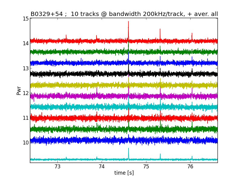
Fig.11 - zooming into 200kHz channels

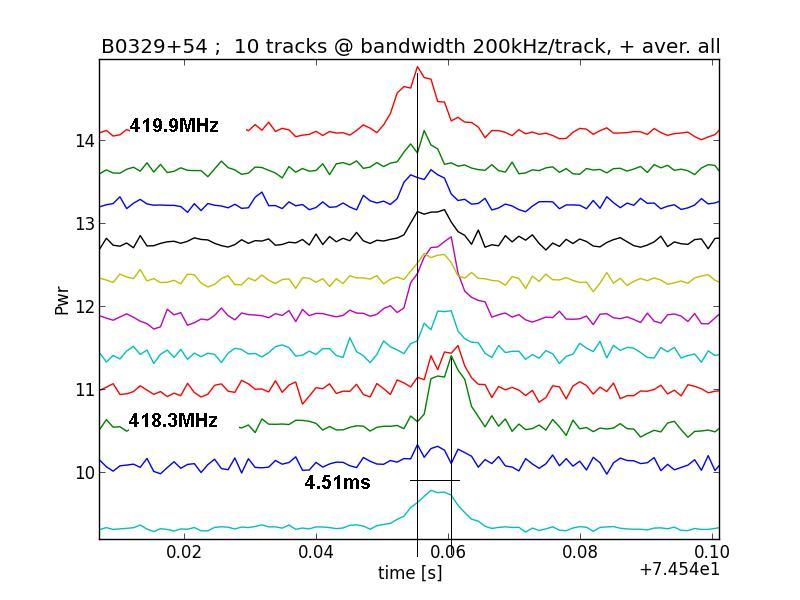
Fig.12 - zooming further into 1 pulse

Now we see that the channels are shifted in time; The lower frequency signals are received later than the higher frequencies.
This is called dispersion, and is caused by the interstellar free electrons.
It is thesame effect as with whistlers
From the graph we can calculate that the delay time is 4.51ms. Now the Dispersion Measure (DM) can be calculated for this pulsar with the following equation;
DM=A3/(B3*(1/C3^2-1/D3^2)) with A3=0.00451s, B3= a constant= 4148.808, C3=freq(low)=418.3MHz, D3=freq)high)=419.9.
This gives us DM=25.0 pc/cm-3
When you compare that with the official value here, it is stated that the DM is 26.77600, so our result is not bad.
Again the accuracy can be improved when more measurements on the other pulses are taken and averaged.
In 1980 the accepted electron density towards the pulsar was tought to be between 0.021 and 0.014 electrons per cm3. This will give you a distance D=DM/ne; between 1.2 and 1.8 kpc.
At the present time the distance can be accurately measured by parallax and now the distance is measured to be 1.03 kpc.

Note that the low frequency channel signal (418 to 418.2MHz) is weak; this is still investigated further.

To correct the delay caused by the inter stellar space electrons we have to un-delay the low frequency cannels.

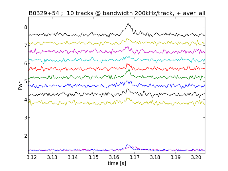
Fig.13 - de-dispersed channels

Zooming in to the averaged result, we see (blue line) that the width of the pulse is smaller and the hight of the pulse becomes larger.

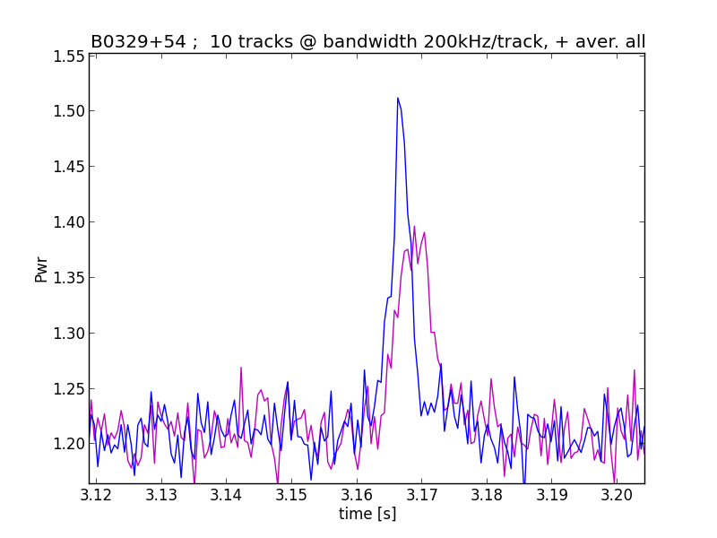
Fig.14 - de-dispersed 9 channel averaged pulse (blue)

Now we can stack again the de-dispersed periods in thesame way as we did with the dispersed periods; fig.15.

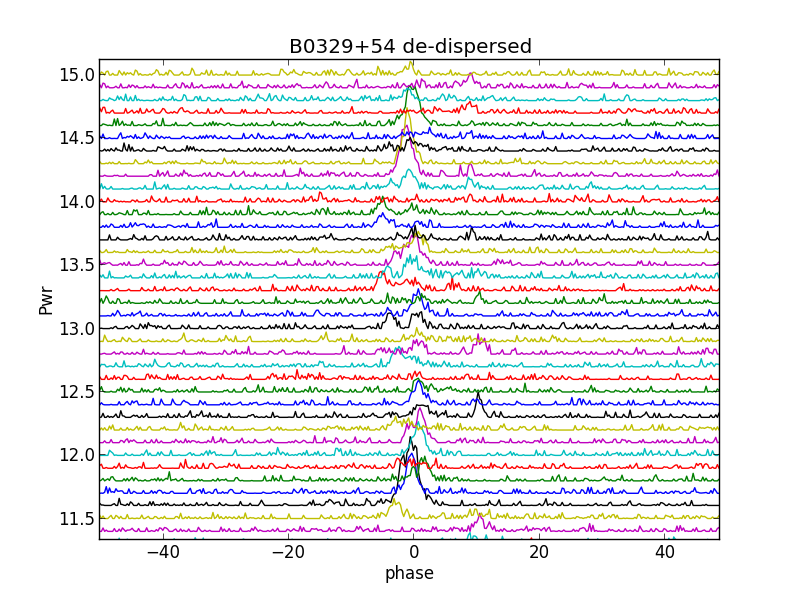
Fig.15 - stacked de-dispersed periods

Because of the de-dispersion, the peaks are sharper now and not blurry wide. We see now more clearly, that there are multiple peaks alongside of each other. This is not caused by a jumpy oscillator of the dongle, because there are more than 1 peaks in the period; higher and wider than noise. So, there must be more emitting area's above the pulsar's magnetic pole.
When we add up selected periods 111 to 129, then we see all the emitters at once. For cosmetics 5 successive data points are averaged. see fig.16

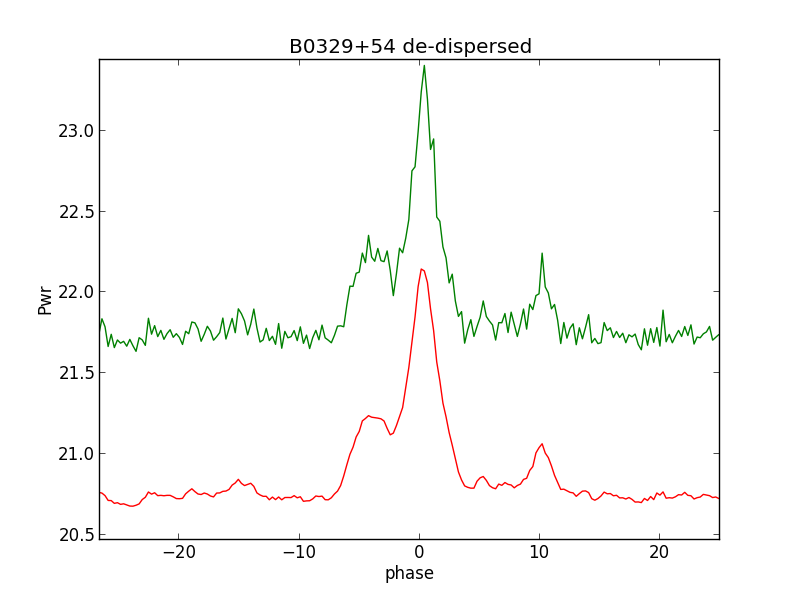
Fig.16 - multiple emitters

So, this result was obtained by adding a selection of periods. If we would have averaged all periods, then the details would not be visible.
The main peak is so strong that smaller peaks are lost when averaging. This method is also called window-threshold technique, and is used in the scientific pulsar detection discipline more.
See here and here
We want to compare our result of course to published results, and we found this;

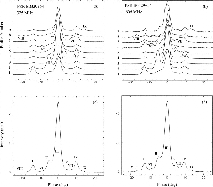
Fig.17 - multiple emitters (Gangadhara and Gupta)

The paper with fig.17 can be found here
Comparing, we can verify the emitting regions I-II-III-IV-V-VII with our own measurements.
In the paper the structure of the emitters is thought to be multiple cones around a core. In another paper it is proposed that the emitters could be a weavering fan like shape.
See here

Let us concentrate on the first idea; the multiple or nested cones. How could it look like in reality. Often a drawing is found like fig 18 and 19.

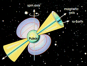
Fig.18 - Pulsar (c) NASA

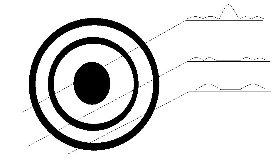
Fig.19 - Line of Sight sweeps

Up to now the theory and the observations agree, however, the pulses drawn in fig 19 are not always there. Sometimes the center pulse disappeares (nulling), sometimes the leading or the trailing pulses become larger or smaller for some time; the so called mode changing, and sub pulse drifting.
There is no accepted explanation for that. A scientist said "we know that a pulsar pulses, but we do not know how".
See the paper of professor Joanna M. Rankin; "The phenomenology and the problem of pulsar emission"; here
A simple measurement of these mode changes can be found here

It is beside the main issue, but in that last paper thier data is not de-dispersed, while measuring with a bandwidth of 1MHz at 327MHz, and a BW of 2MHz at 610MHz.
The W50 ( that is the width of the main pulse at 50% of the max value) is measured to be 3.9 and 3.2 degree respectively.
Our de-dispersed measurement at 419MHz gives us a W50 bandwidth of 4.3ms or 2.2 degree.
In the VizieR data base; http://vizier.u-strasbg.fr/viz-bin/VizieR-S?PSR%20J0332%2b5434 for W50 a value of 6.6ms is given. There is no further info of Band Width or tuning frequency.


Radiating diameter.
Earlier we have calculated the maximum possible diameter of the pulsar, however with other calculations it is determened that the radius is about 10km.
As an approximation we can calculate what the surface diameter is of the area where the radio signal is could be generated.
With W50=2.2 degree, R=10km and the radiating surface on the surface we get;
Radiating diameter rd=2*pi*R*2.2/360=366m.
The electrons guided by the field lines spiral down because of the huge gravity, and collide on their way toward the area with other particles to generate photons.
Lower frequencies are generated higher up the funnel, higher frequencies upto gamma rays are generated lower in the "horn".

By studying hundreds of reports of pulsars, the above mentioned J.M.Rankin discovered patterns in the results.
She has written a series of papers called "Toward an empirical theory of pulsar emission" I to XI ; IV here, in which graphical results could be turned into approximating formula's.

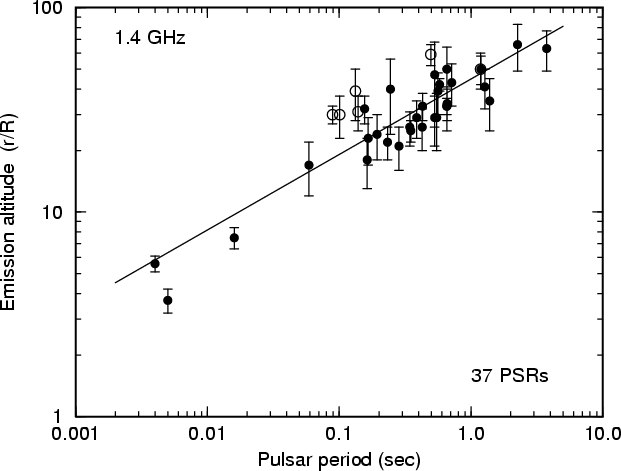
Fig.20 - emission altitude as function of period time

Inclination angle.
For instance in paper IV the inclination angle ( the angle btween the rotation axis and the magnetic pole axis) can be calculated.
Alpha=arcsin(2.45/(W50*sqrt(P))=29[deg], where P is the period=0.714s, and W50 is the pulse width at 50% hight=2.2 deg.

Emission hight.
Another approximation is the calculation of the location hight of the emission .
The original data was obtained by measuring the small differences in time of arrival (TOA) of the radio signals on different frequencies.
r/R=45*Pexp(0.37)=45*0,714*EXP(0,37)=47, valid for old pulsars, where R= pulsar Radius=10km, P=period time =0.714s
So the radio emission of B0329+54 on 430MHz is originating at 47*10[km].

For 1.4MHz the hight ratio is r/R=35*Pexp(0.37)=35*0,714*EXP(0,37)=36; giving r=36*10 [km]

Gamma rays are originating at 1.8*R.

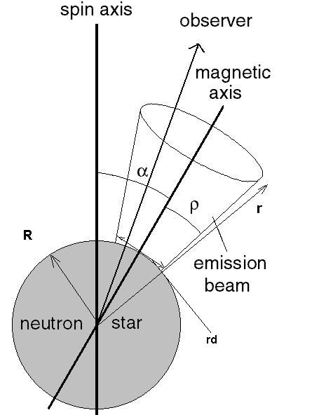
Fig.21 - Alpha and Emission altitude

Michiel Klaassen march 2016