[HOME]   [WEB ALBUMS]   [PROJECTS]   [ARCHIVE]   [DOWNLOADS]   [LINKS]  



PROJECTS



Project MK1: Sampling 21cm neutral hydrogen signals with a Velleman digital oscilloscope.

As radio astronomy amateur, I wondered if, with very simple electronic equipment, but with the 25m Dwingeloo Telescope (DT) a 21cm measurement was possible.

The report of the Frans de Jong and Paul Boven is known. They have measured the Andromeda nebula and done an all-sky scan measurements at 21 cm. However his this was done with a backend and software normally not available to amateurs. The backend is a fast AD converter and FPGA programmed for rapid sampling, FFT processing and averaging of data. There are similar SDR (software defined radio) systems available, but these are expensive.

The idea was to use ready available instruments for these 21cm hydrogen measurements. So it was decided to do an experiment with a simple amateur digital oscilloscope, the PCS500 from the company Velleman.

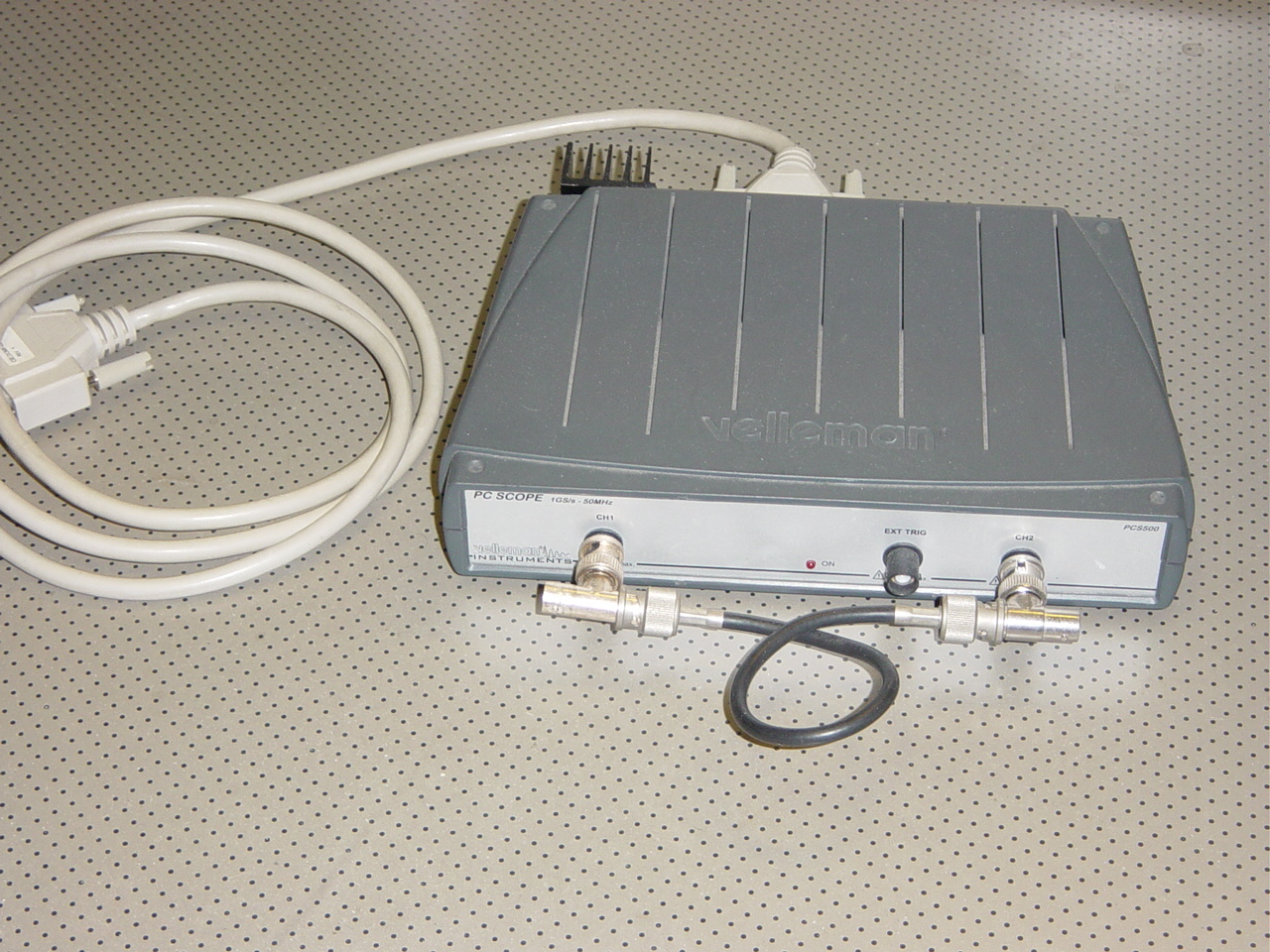
Fig.1 - Velleman digital oscilloscope type PCS500.

This digital scope must be connected with a parallel cable to the PC and can sample two channels. The new versions have usb interfaces, but this old one was laying unused on the shelf. The maximum sampling rate is 1GS/s (for synchronous signals) and up to 50M Samples per second asynchronous. After FFT this gives a signal bandwidth of 25 MHz.Other settings are 12MS/s, 3MS/s, 1.25MS/s etc., each resulting in a signal bandwidth of 6, 1.5, 0.625MHz etc.

First observation session. The sampler was first connected to the existing Rohde and Schwarz receiver in the DT.

The telescope is aimed at the coordinates RA 21H11m12s, and DEC 45d41m51s. This can be converted to the galactic coordinates L = 88.3517, b =- 1.787. That means we see the galaxy at about 90 degrees to the left of the galactic center, and about 2 degrees below the rim.

All data within the 25MHz band and coming through the R/S panoramic receiver is sampled for one minute and written on the hard disk. For capture and storage a macro basic program was written in Excel. For this capturing, a Velleman free DLL was used with Excel. On disk this will give you a file of 4096 x 8 bit data values, preceded by three values which are the sample rate, the full scale value in mV, and the zero line value . Of course, also important is the refresh rate, and this is about 50ms because we want to get as much frames as possible . The Excel macro is set to loop now 1000 times to acquire a frame of 4099 values and save it. The total actual measurement time is 80ms.The total capture and disk writing time is 52secons; so the time efficiency is 0.15%. Ultimately, only one measuring session, set to 50MS/s was successful, giving a total of 25Mbytes of data. Other attempts in that session have failed.

This data must now be analyzed at wavelength content. This can also be done with excel, FFT calculations using the subroutine "ATPVBAEN.XLA! Fourier". For broadband noise signals it is not necessary to use windowing. Windowing is a way to treat the signal like, with a switch on / off from the "speaker", or with a potentiometer turned from zero to maximum and back to zero again. Because the raw data is stored is always possible to recalculate with a Hanning, Gaussian or Welch window later. For each of the frames of 1000 times 4096samples the frequency spectrum is calculated, then summed and averaged.

The result of the calculation gives a frequency spectrum. However, the Excel calculation lasted 2.5 hours. A faster PC did not give much extra approximately 2xthe speed of the first. Then we were assisted by the Portuguese amateur astronomer Ricardo Gama, who has written a python program, and we got the result in 30sec.

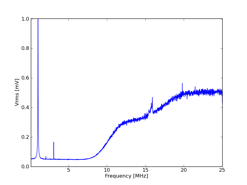
Fig.3 - First Light Hydrogen.

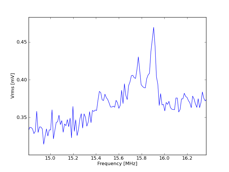
Fig.4 - Close up.

On the graph the first part of the bandpass filter of the receiver can be seen beginning at approximately 10MHz. On 1MHz there is a reference signal, and on 15MHz the actual 21 cm profile signal. The efficiency of the bandwidth is low, approximately 1 / 25 = 4%. One can magnify the signal, but this does not give a better resolution. Also note that the frequency spectrum of the line is reversed, this reversal is due to the R/S Receiver. The conclusion is that we can use this sampler, but the measurement must be improved.



Second observation session.

Now we know that the sampler works, we want the most effective measurement possible. The 21cm signal is about 2 MHz wide, so we try to get it directly from the receiver.

We do not want to use the R/S receiver, but we can use a communication receiver Yaesu VR5000.

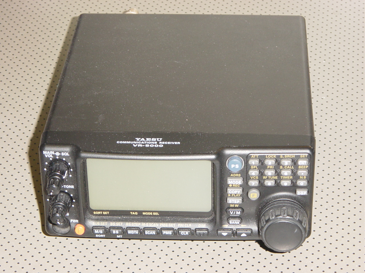
Fig.5 - Yaesu Receiver.

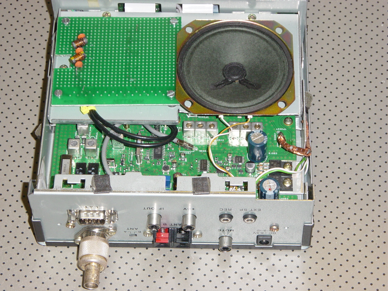
Fig.6 - Yaesu open.

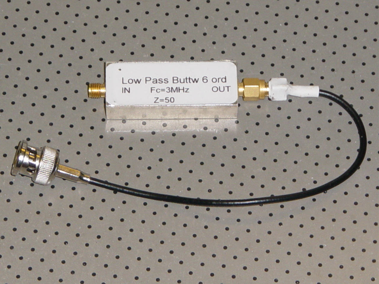
Fig.7 - Lowpass Filter 3MHz.

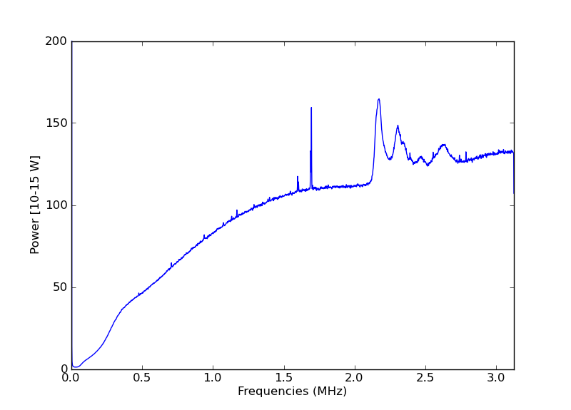
Fig.8 - 50000 spectra.

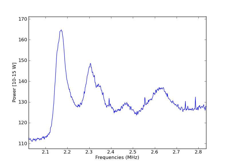
Fig.9 - Detail.