[HOME]   [WEB ALBUMS]   [PROJECTS]   [ARCHIVE]   [DOWNLOADS]   [LINKS]  



PROJECTS





Project EM01: Mini maser telescope: detecting 12.2 GHz methanol masers with a 1-metre dish

In recent years, the hydrogen line at 1420.405 MHz has become a popular target for amateur radio astronomers. It is a relatively strong signal (at least compared to other natural sources), it is everywhere in the sky and can easily be detected with low-cost equipment. It is therefore not surprising that the majority of amateur radio astronomy focuses on the hydrogen line. However, there are many more lines in the radio spectrum, and with some effort it is possible to detect at least a few of them. On this webpage, I will describe how I detected 12.2 GHz methanol masers with a small dish.

You may not be familiar with methanol masers. Very short description: methanol masers are a particular type of radio source found in star forming regions. They emit unusually bright spectral lines of the methanol (CH3OH) molecule. One of these spectral lines is the transition at 12178.593 MHz, ant that is what we try to detect. For further information about these objects I will refer to Michiel’s pages about methanol masers on this website (see project pages MK21- MK24).

So how did this project get started? I have been doing amateur radio astronomy since late 2017. I first learned about methanol masers from Michiel’s webpages. Michiels results were very impressive and interesting but he did his measurements using a 9.3(!) metre dish. Obviously the average amateur does not have access to such large equipment. However, linked under one of Michiels webpages I found a memo of the VSRT/ MOSAIC project by the Haystack observatory, describing the feasibility of detecting methanol masers with much more modest size dishes [1]. They calculated using the radiometer equation that a dish as small as 1.2 metres could already detect the few strongest methanol masers with tens of minutes to a few hours of integration time. However, the values they used were still rather optimistic (such as 70% aperture efficiency; we are already very happy with 40 to 50%) so it may be much more difficult and time- consuming in reality… but still worth a try!

Wat do we need to detect methanol masers? Fortunately, most parts are not too expensive and readily available. As discussed in the Haystack VSRT memo, a 1.2 metre dish should theoretically be sufficient to detect the few strongest methanol masers. Unfortunately, when I started working on this project I could not easily obtain a dish of 1.2 metres or larger. Therefore, a slightly smaller 1.1 by 1 metre offset dish was purchased instead.

In order to do observations the dish needs to be accurately pointed at the target. It is possible to simply set the dish at the declination of the target and let the target drift through the beam every day. However, it would take several weeks to gather a few hours of integration time with this method. It is therefore preferable to put the dish on a mount which can track the source. For this a HEQ5 equatorial mount was used, which I normally use for astrophotography. The 1 metre dish was not too heavy for this mount.

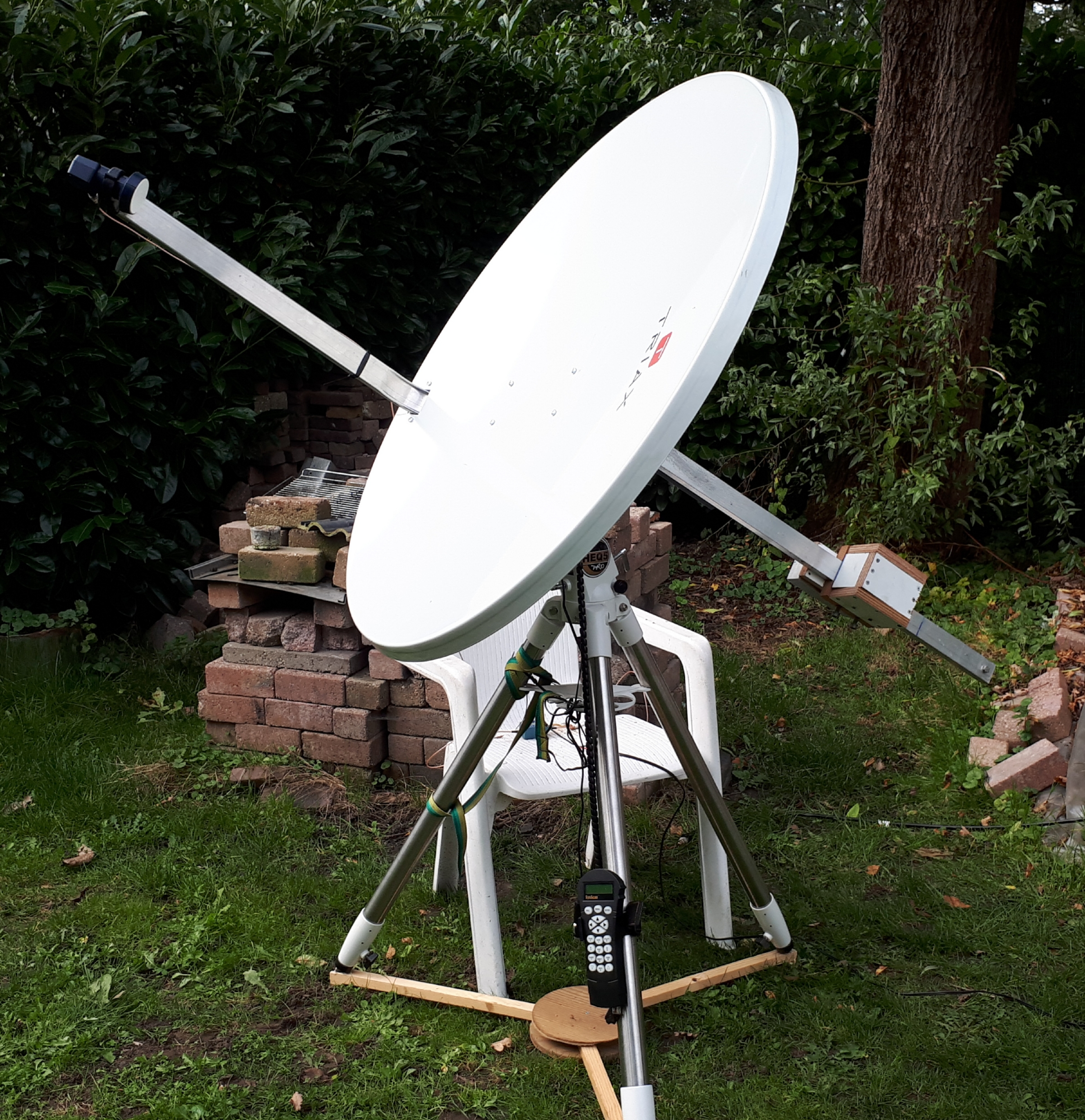
Fig.1 - 1 metre offset dish mounted on HEQ5

Unfortunately, while the tracking worked perfectly with the dish on the mount, pointing the dish was still not an easy task. The offset dish “looks” in a different direction than where the mount is pointing it, and because of this the GoTo system of the mount did not point the dish in the right direction. For the time being it was decided to use the old-fashioned method of star hopping. A small finder scope from my telescope was attached to the side of the dish. It was aligned with the beam of the dish by slewing to the Moon until I had maximum moon noise, and then adjusting the orientation of the finder until the Moon was in the crosshairs of the finder. To point the dish to a target, a star map of the area around the target (including the nearest bright star) was generated using Stellarium. I then started off from the nearest bright star, and star- hopped to the position of the target using the star map. A drawback of this method is that the dish cannot be pointed at daytime this way, so observations are restricted to night time. Proper alignment of the dish with the mount so that setting circles or the GoTo system can be used is an improvement for the near future.

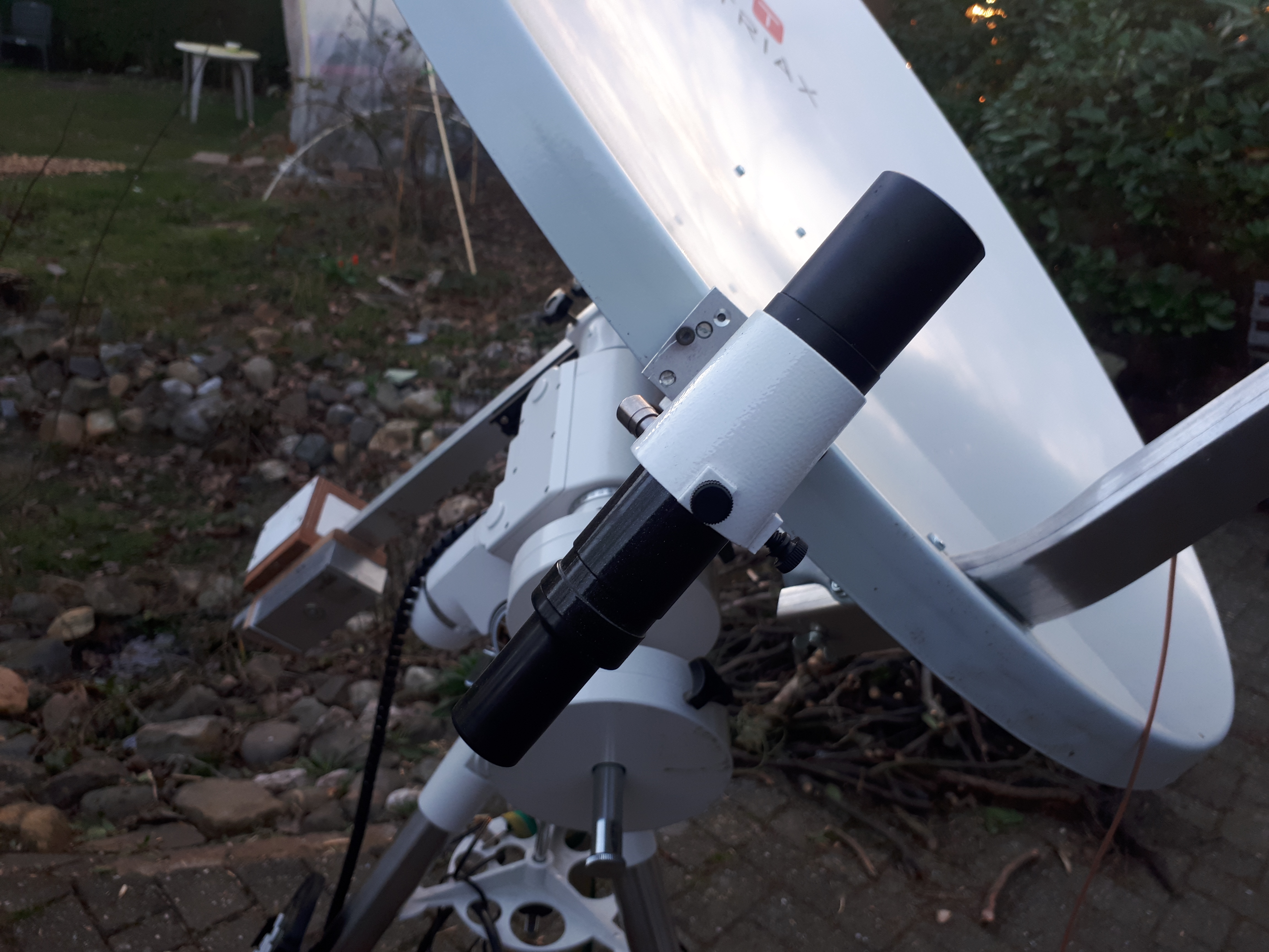
Fig.2 - finderscope attached to the side of the dish

Next thing we need is a downconverter or LNB. Michiel has had success using a standard Ku band LNB. However, he also noted that frequency drifting (due to the LNB heating up and cooling down) was a major problem, especially with non-PLL (e.g. DRO-type) LNBs. The problem was much less for PLL LNBs, but even these had some drift. He eventually solved the frequency drifting problem by locking the LO to an external reference (see project MK21). However, I was going to do my first observations at night, when temperature variations are relatively small. Because of the smaller dish (and therefore much weaker signal) it was decided to use a lower resolution of about 5.8 KHz to get a higher SNR. The maser lines are generally more than 10 KHz wide, so if the LNB drifted by 10 KHz or less stability was deemed sufficient. To test whether my LNB could be used without any modification, I took measurements of a satellite beacon for several hours and looked how much the frequency varied/ drifted.

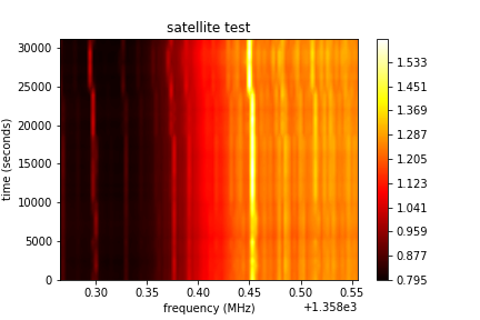
Fig.3 - LNB drift test.

From these tests it was concluded that the LNB LO drifted by about 10 KHz once it had cooled off to the temperature of the surroundings. This was sufficiently stable for at least my first experiments.

The LNB has two different LO’s: a low band LO at 9750 MHz and a high band LO at 10600 MHz. For detecting the methanol line at 12178 MHz, I needed to switch on the high band LO. The methanol line frequency is then converted down to 12178-10600=1578 MHz, well within the frequency range of my airspy mini SDR. Band switching is done by inserting a 22 KHz tone. Since I am not that experienced with electronics myself, I am very grateful to my father for building a special power supply from standard components. It provides 12V DC to power the LNB with the 22KHz tone for band switching superimposed. This is fed to the LNB via a bias tee.

Now we were ready to detect our first maser. The antenna temperatures of the strongest masers with 1 metre aperture are in the order of 100- 200 millikelvins. This is about 1000 times less than the system temperature! It is therefore needed to record multiple hours of data to achieve a sufficiently high SNR. For this I used SDR# with the IF average plugin written by Daniel Kaminski. I let IF average save a spectrum every 2- 3 minutes as a .txt file. It should be noted that IF average is not the most efficient FFT averaging software, but this did not seem to be a huge problem otherwise the observations would have failed. Often observations were spread over multiple days, collecting spectra of the target for two or three hours per day. All these spectra were averaged later on to achieve a higher SNR.

The bandpass response of the SDR is also not at all flat. It is needed to correct for the bandpass response just like for HI observations. Therefore a number of “off-target” or “dark” spectra have to be recorded with the same setup and preferably under the same circumstances while the dish is pointed away from the target. These off-target spectra should have the exact same bandbass response but without the signal. After dividing or subtracting this “off-target” spectrum from our “on-target” spectrum which contains the signal we are interested in, we should be left with just the signal and not the bumps and crests caused by the SDR.

In order to get good SNR it is needed to record dark spectra for at least the same amount of time that was used to record spectra of the target. “Dark” spectra were made by pointing the dish away from the target. Bandpass correction is done by averaging all the “dark” spectra and dividing the spectra of the target by the averaged dark. After that there is often still some residual slope, this is corrected for by fitting a line through the points outside a defined window were the spectral line is, and then dividing the spectrum by this line.

Finally, after each observing session a spectrum of the Astra 3B satellite beacon at 11446.7266 MHz was recorded. This was used for measuring and correcting the LO offset. Above I mentioned that the LO did not drift too much, but there was still often a significant frequency deviation. By measuring a beacon with a known frequency, it was possible to determine by how much KHz the LO was offset and subtract the offset from the frequency values. After LO offset correction the frequency values were used to calculate radial velocity values using the Doppler formula. For Vlsr correction the ATNF frequency/Vlsr calculator [2] and the Vlsr calculator of Steve Olney [3] were used.

The first results were from the methanol maser in the star forming region W3(OH). This is also one of the strongest methanol masers with a flux density of about 800 Jy. There are multiple overlapping features in its spectrum between -42.5 and -45.5 kms [4]. W3(OH) was observed six times for 1.5 to 3 hours per session between February 20 and 27, 2021. After processing the vast amount of collected spectra as described above, a signal was found in all of the averaged spectra of the six observation runs. This signal was at approximately the expected velocity for W3(OH). The SNR varies a bit between different runs but this could be attributed to different integration times for each run.

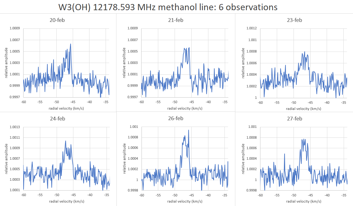
Fig.4 - W3(OH) 6 days of observations

However, there was still a velocity offset of about 2 km/s. This meant that either something was going wrong with my LO frequency offset correction or velocity calculation, or the signal was a very persistent form of RFI that happened to be around the expected frequency for W3(OH).

In a post on the SARA forum Wolfgang Herrmann suggested that I should check the Vlsr correction. I initially used the online calculator on the ATCA website [2]. The results of the ATCA calculator were compared to the results of Steve Olneys Vlsr calculator [3], which was proven to be fairly accurate in the past. The results of the two calculators only differed by about 300 m/s. This small difference was not enough to account for the 2 km/s discrepancy.

The next thing that could be a problem was the LO frequency offset correction using a satellite beacon. For this a beacon of the Astra 3B geostationary satellite was used. According to the beacon catalogue on UHF-satcom.com [5] this beacon is at 11446.800 MHz. However, another source (frequencyplansatellites.org) listed this beacon at 11446.75 MHz. None of these are “official” sources, both are compiled and maintained by amateurs so it was suspected that there was some uncertainty on the beacon frequency. In order to figure out the exact frequency of the beacon, it was compared to a beacon with a known frequency. For this the beacons marking the downlink band of the eshail2 satellite’s amateur radio transponder could be used. These are at 10489.500 and 10489.750 MHz according to Amsat-dl [6] Unfortunately this is too low to be received with the high band LO turned on. Hence, I did not use these beacons instead of Astra for LO frequency offset measurements after my methanol maser observations. Fortunately both the Astra 3B beacon and the Eshail2 beacons fall within the range of the low band LO, so they could still be used to pin down Astra 3B’s frequency. The Eshail beacons were used to measure the LO frequency offset, and this frequency offset was subtracted from the measured frequency of Astra 3B to get its true frequency. This turned out to be 11446.7266 MHz; quite far off from the frequencies listed in both sources!

With the correct frequency of the Astra 3B beacon now finally measured, the whole LO frequency offset correction of all previous W3(OH) observations was done over. At this point a small error in the spreadsheet used for frequency correction and velocity calculation was also found and corrected. (Yes I used Excel for this, given the low number of observations I did not feel urged to write a separate python script for it at this point)

With these problems now solved, the velocity of my signal was spot- on for W3(OH)! As a final test W3(OH) was re-observed at March 19, nearly a month after the first observation run. If the signal we see is indeed from a celestial source like W3(OH), we expect to see a slow velocity shift due to Earth’s orbit around the Sun. However, we correct for this velocity shift when we calculate the LSR velocity. The signal should therefore stay at exactly the same LSR velocity no matter the time of the year when it is observed. If it does not, then the signal is most likely manmade interference. I was therefore very pleased to see that the spectrum taken at March 19 still showed the same signal at the same LSR velocity.

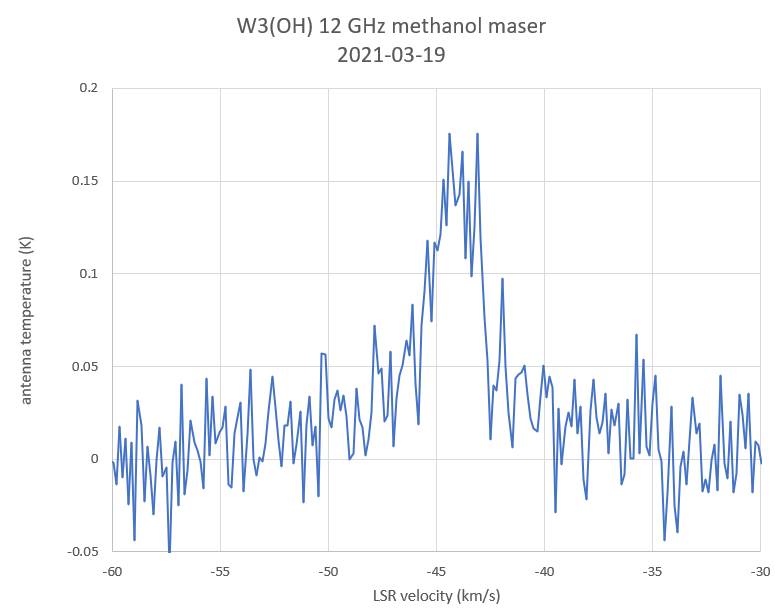
Fig.5 - W3(OH) March 19, 2021

Finally, all the results of these seven successful observation runs were averaged to achieve a better SNR. This was nearly 17 hours of measurements! The averaged end result revealed four different features in the spectrum at -43, -44.3, -44.7 and -45.4 km/s.

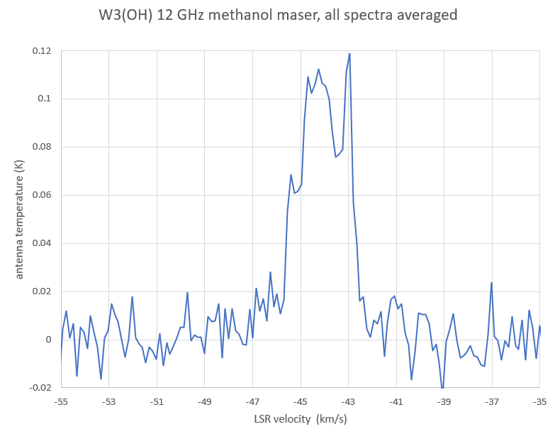
Fig.6 - W3(OH) all spectra averaged

We can compare this spectrum to the spectra of W3(OH) obtained by Michiel Klaassen with his 9.3 metre dish between 2016 and 2019 (see project MK23). In these spectra the same four features can be recognised. It appears that the feature at -43 km/s is a bit stronger in my spectrum while the feature at -45.4 km/s is weaker. This could be due to the lower SNR of my spectrum but the intrinsic variability of the maser could also play a role. In Michiels spectra it can be seen that the intensity of these features indeed varied between 2016 and 2019. If the variations recorded by Michiel are real and not an instrumental artefact, we would indeed expect to see some changes after a few years.

After the very successful detection of W3(OH) I wondered whether there are more methanol masers accessible with my small dish. One of the potentially detectable targets was G188.94+0.89, hereafter G188. However, G188 has a flux density of around 200 Jy- it is four times weaker than W3(OH). Its LSR velocity is +10.9 km/s [4]. Four observation sessions (about two and a half hours for each session) were done in an attempt to detect this maser. There was indeed a very small peak at around 11 km/s in the averaged spectra from March 23, 25 and 29. However, this peak was absent in the data from March 27.

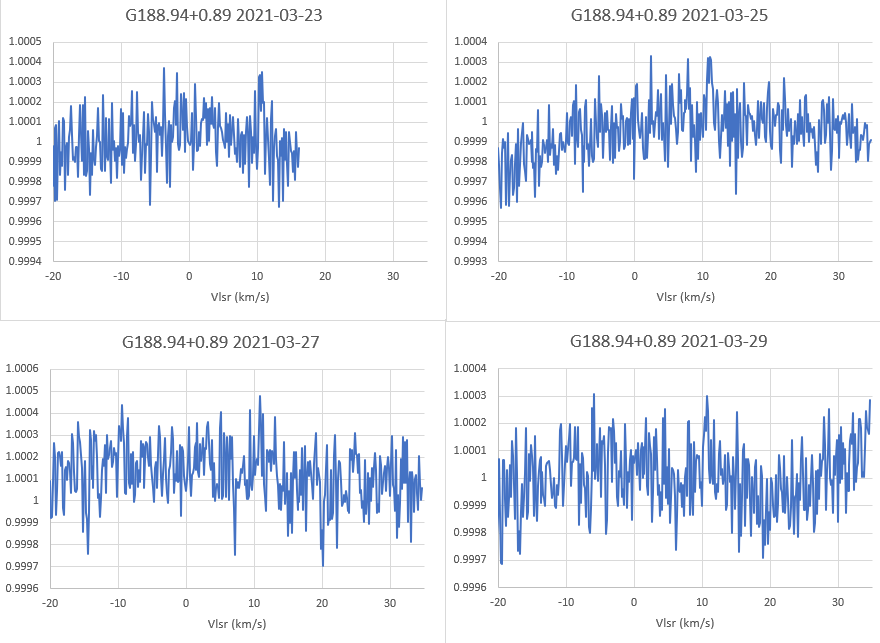
Fig.7 - G188 observations

Michiel noted that his observations at 12GHz were often degraded when it was overcast. Indeed, clouds rolled in early during the observation session on March 27. For such a weak signal, even a small attenuation and increase in system temperature due to clouds could result in a non-detection. It was therefore decided not to use the data of March 27 and averaged all spectra from the other observing sessions. To increase the SNR, each FFT bin was averaged with the previous and the next bin. This effectively reduces spectral resolution from 5.8 KHz to 17.4 KHz, but that is not a problem as long as the spectral line is sufficiently wide.

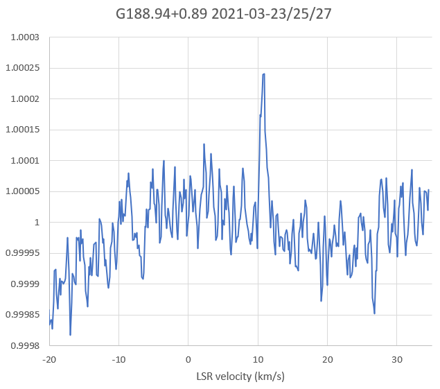
Fig.8 - G188 all spectra averaged

In the resulting averaged spectrum, the peak at 10.9 km/s is clearly visible. The SNR is a bit low (about 5.1), but that was to be expected. The peak is at the right velocity and was detected three out of four times, so this still seems a positive detection. The spectrum is not at all flat, it seems to be very difficult to get a good flat spectrum with bandpass calibration when attempting to show such weak signals.



references:

1): VSRT memo 065, 21 September 2009: “On the feasibility of a low-cost methanol telescope”, Vincent L. Fish & Alan E. E. Rogers.

2): ATNF frequency calculator, Bob Sault 2004: https://www.narrabri.atnf.csiro.au/observing/obstools/velo.html

3): HawkRAO Vlsr calculator by Steve Olney. (No longer online)

4): Catarzi, M., Moscadelli, L., & Panella, D. (1993). Observation of methanol maser sources with the Arcetri 12 GHz receiver. Astronomy and Astrophysics Supplement Series, 98, 127-135.

5): UHF-satcom satellite reception; Ku band frequency list: https://uhf-satcom.com/satellite-reception/ku-band

6): P4-A NB transponder bandplan and operating guidelines: https://amsat-dl.org/en/p4-a-nb-transponder-bandplan-and-operating-guidelines/





Eduard Mol july 2021

eddiemol2000@gmail.com